Leaflet in R
This post shows how to build beautiful interactive maps in R using leaflet.
library(leaflet)
library(sf)
library(terra)
library(raster)
library(RColorBrewer)
library(htmlwidgets)
Read data
Here I am reading three different datasets, a polygon (mx_states) and a point (caps) layer, as well as a raster (DEM).
# States polygons
# Data downloaded from http://www.conabio.gob.mx/informacion/gis/?vns=gis_root/dipol/estata/dest22gw
mx_states <- st_read("dest22gw.shp")
# DEM
# Data downloaded from: http://www.conabio.gob.mx/informacion/gis/?vns=gis_root/dipol/estata/dest22gw
dem <- rast("filled_demgw.tif")
# Capitals
# Data downloaded from: https://www.efrainmaps.es/descargas-gratuitas/m%C3%A9xico/
caps <- st_read("México_Ciudades.shp")
Create palettes
Create palettes for the data. Here we are goin to use RcolorBrewer functionalities and some leaflet functions. Also, notice that I am creating two palettes for the DEM. This is a small hack to put the legend in a reverse order (low values in the lower side and higher in the upper one).
## States palette
coul <- brewer.pal(4, "PuOr")
pal_st <- colorRampPalette(coul)(33)
## Dem palette
coul <- grDevices::colorRampPalette(c("#026449", "#12722c","#d7d17e",
                                        "#95400d", "#980802", "#746c69", "#f1f1f1","#fdfdfd"),
                                      interpolate = "spline",
                                      bias = 1)(256)
pal_dem <- leaflet::colorNumeric(
  c("#026449", "#12722c","#d7d17e",
    "#95400d", "#980802", "#746c69", "#f1f1f1","#fdfdfd"),
  values(dem),
  na.color = "transparent",
  alpha = FALSE,
  reverse = FALSE
)
# Palette hack to invert legend
pal_dem2 <- leaflet::colorNumeric(
  c("#026449", "#12722c","#d7d17e",
    "#95400d", "#980802", "#746c69", "#f1f1f1","#fdfdfd"),
  values(dem),
  na.color = "transparent",
  alpha = FALSE,
  reverse = TRUE
)
## Capitals palette, same as states
Leaflet map
Then create the leaflet map. First let’s add the polygons.
mapa <- leaflet::leaflet()

## Add Polygons
mapa <- mapa %>%
    leaflet::addPolygons(data = mx_states,
                         stroke = TRUE,
                         smoothFactor = 0.5,
                         opacity = 1,
                         fillOpacity = 0.9,
                         fillColor = ~ pal_st,
                         weight = ~0.2,
                         color = ~"black",
                         group = "States",
                         popup = ~mx_states$NOMGEO)
Add the raster. Here notice the use of pal_dem2 in addLegend and sort the values in decreasing order using labFormat.
## Get tange of dem
minmax <- range(raster::values(dem)[!is.na(raster::values(dem))])

## Add raster
mapa <- mapa %>%
  leaflet::addRasterImage(raster::raster(dem),
                          colors = pal_dem,
                          opacity = 0.9,
                          group = "DEM",
                          layerId = "DEM") %>%
  leaflet::addLegend(position = "bottomleft",
                     pal = pal_dem2,
                     values = seq(minmax[1], minmax[2], 100), #4 categorical maps terra::levels(dem)[[1]]$ID,
                     title = "Elevación m s.n.m",
                     labFormat = labelFormat(transform = function(x) sort(x, decreasing = TRUE)))
                    # for categorical maps
                     # labFormat =  leaflet::labelFormat(
                     #   transform = function(x) {
                     #     df_eq %>%
                     #       dplyr::filter(ID == x) %>%
                     #       dplyr::pull(!!sym(key))
                     #   }))
Add the points. Here I set a different color to the circle inside the marker.
## Points
### Create customized markers
### Can create in several lists, that's why two lapply are used
### In this case we really only need one level
resul <- lapply(1:length(pal_st), function(j){
    leaflet::makeAwesomeIcon(
      icon = "circle",
      library = "fa",
      iconColor = pal_st[j],
      markerColor = "white",

    )
  })
# Cast as awesome icon list
resul <- structure(resul, class = "leaflet_awesome_icon_set")

## Add points
mapa <- mapa %>%
    leaflet::addAwesomeMarkers(data = caps,
                               icon = resul,
                               popup = ~caps$CIUDAD,
                               group = "Capitals")
Add three Esri basemaps
## Base maps
mapas_base <- c("Esri.WorldTopoMap", "Esri.WorldImagery", "Esri.WorldGrayCanvas")

# Add basemaps
for(provider in mapas_base) {
  mapa <- mapa %>%
    leaflet::addProviderTiles(provider,
                              group = provider)
}
Add controls and mini map. OverlayGroups should match the name given for each layer in the previous sections.
# Add controls and mini map
mapa <- mapa %>%
  leaflet::addLayersControl(overlayGroups = c("States", "DEM", "Capitals"),
                            baseGroups = mapas_base,
                            position = "topright",
                            options = leaflet::layersControlOptions(collapsed = FALSE,
                                                                    hideSingleBase = TRUE)) %>%
  leaflet::addMiniMap(tiles = mapas_base[[1]],
                      toggleDisplay = TRUE,
                      position = "bottomleft")
Add more customizations: change base map, zoom to extent of layers, add globe button to reset zoom level to the starting point, add opacity slider.
# More customizations
mapa <- mapa %>%
  # update base map
  htmlwidgets::onRender("
    function(el, x) {
      var myMap = this;
      myMap.on('baselayerchange',
        function (e) {
          myMap.minimap.changeLayer(L.tileLayer.provider(e.name));
        })
    }") %>%
  # add full extent button
  leaflet::addEasyButton(leaflet::easyButton(
    icon = "fa-globe",
    title = "Zoom to Level 1",
    onClick = leaflet::JS("function(btn, map){ map.fitBounds([
                                        [", 14.55712, ",", -117.12579, "], ",
                          "[", 32.71876, ",", -86.74011, "]
                                        ]); }"))) %>%
  # opacity slider
  leaflet::addControl(html = "<input id=\"OpacitySlide\" type=\"range\" min=\"0\" max=\"1\" step=\"0.1\" value=\"0.5\">") %>%
  # change opacity of the layers
  htmlwidgets::onRender(
    "function(el,x,data){
                     var map = this;
                     var evthandler = function(e){
                        var layers = map.layerManager.getVisibleGroups();
                        console.log('VisibleGroups: ', layers);
                        console.log('Target value: ', +e.target.value);
                        layers.forEach(function(group) {
                          var layer = map.layerManager._byGroup[group];
                          console.log('currently processing: ', group);
                          Object.keys(layer).forEach(function(el){
                            if(layer[el] instanceof L.Polygon){;
                            console.log('Change opacity of: ', group, el);
                             layer[el].setStyle({fillOpacity:+e.target.value});
                            }
                          });
                        })
                     };
              $('#OpacitySlide').mousedown(function () { map.dragging.disable(); });
              $('#OpacitySlide').mouseup(function () { map.dragging.enable(); });
              $('#OpacitySlide').on('input', evthandler)}
          ")
Save file as html widget.
htmlwidgets::saveWidget(mapa,
                        "Map1.html")
The final result (click on the following image to access the map):
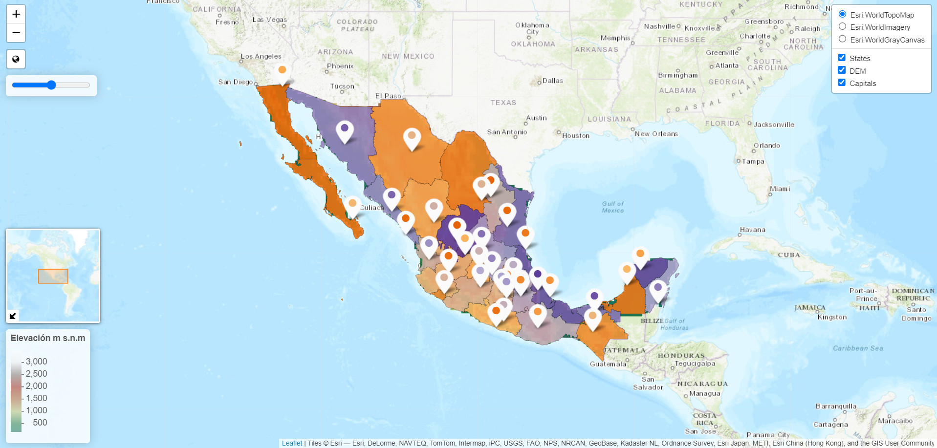 Interactive leaflet map.