Volcanos 3d maps
I have continued playing with rayshader, rayvista and magick packages to make beautiful 3d maps. This post shows the code used to make a 3d map with some of the highest peaks in Mexico, which all have a volcanic origin. Additionally, the area shown in the map is part of the Trans-Mexican Volcanic Belt. The code used to obtain this map is shown in the first section. The second section of the post contains the code used to make the zoom-ins to each volcano, while the third section contains the code used to merge all the images.
First load the required packages.
library(rayvista)
library(rayshader)
library(terra)
library(dplyr)
library(sf)
library(magrittr)
library(magick)
Load the roi polygon to make the large map and also a geopackage file that contains points with the locations of each volcano, with its name and altitude. Although initially I wanted to label also Sierra Negra peak, it was overlapping with the Pico de Orizaba so I removed it. Then, the coordinates are extracted from that same file, added as columns and then added a color column to indicate the color of the labels (white: for names that overlapped with the rgb composite and black those that did not). Finally, calculate the area to add it in the end as a label. The data used in this example can be downloaded from: https://github.com/JonathanVSV/Ppage2/tree/master/assets/data
# Zscale for 3d map
zscale <- 60
# Background color for all maps
bg_col <- "gray60"

# ROI
picos_poly <- st_read("Data/Picos.gpkg")
# Points of each peak with its name and altitude
picos_names <- st_read("Data/picos_names.gpkg") |>
  # Removed Sierra Negra because was overlapping with Pico de Orizaba
  filter(Name != "Sierra Negra")
# Get its coordinates
coords <- picos_names |>
  st_coordinates()
# Add the coordinates as another column and add a color column
picos_names <- picos_names |>
  bind_cols(coords, color = c("white", "white", "white",
                              "white", "black", "black", "white")) |>
  # Arrange by altitude for the individual volcanos plots
  arrange(desc(Alt))

 # Calculate area in sq. km
areasqkm <- 25000

# Aprox area without zoom
# picos_poly |>
  # st_transform(32614) |>
  # st_area() |>
  # as.numeric() |>
  # multiply_by(1/1000000)
Then, obtain the RGB data with the DEM.
Large map
Obtain rgb composite and DEM data.
picos<- plot_3d_vista(req_area = picos_poly,
                          overlay_detail=10,
                          overlay_alpha = 0.7,
                          elevation_detail=9,
                          show_vista = F)
Then, create the 3d representation and add the labels and save a snapshot of the rendered image.
# Use dem matrix data
picos$dem_matrix|>
  # Add texture
  add_overlay(texture_shade(picos$dem_matrix,
                            detail=0.9)) |>
  # Add snowy peaks effect
  add_overlay(generate_altitude_overlay(height_shade(picos$dem_matrix,
                                                     texture = "white",
                                                     range = c(5000,5700)),
                                        picos$dem_matrix,
                                        start_transition = 4500,
                                        end_transition = 5000,
                                        lower=FALSE),
              alphalayer = 1)  |>
  # Add Shadow
  add_shadow(ray_shade(picos$dem_matrix, zscale=zscale), 0.7)|>
  # Add RGB composite
  add_overlay(picos$texture,rescale_original=TRUE)|>
  # Plot 3d
  plot_3d(picos$dem_matrix,
          zscale=zscale,
          windowsize = 1200,
          zoom=0.17,
          phi=7,
          theta=280,
          background = bg_col)

# Add labels
for(i in 1:nrow(picos_names)){
  # color <- "black"
  render_label(picos$dem_matrix,
               long = picos_names$X[i],
               lat = picos_names$Y[i],
               zscale = zscale+60,
               extent = attr(picos$dem_matrix, "extent"),
               text = paste0(picos_names$Name[i]),
               linecolor = picos_names$color[i],
               textcolor = picos_names$color[i])
}

# Save as png
render_snapshot(filename = "Plots/Volcanos_snap.png",
                software_render = F,
                background = bg_col)
Individual volcanoes
This section contains the code used to make the zoom-ins to each volcano. It contains basically the same code as the previous sections but obtains the DEM and RGB composite using the location of each volcano. Finally, to make everything more easy, an lapply is used to make the exact same process for each volcano and save the rendered image as a png.
lapply(1:nrow(picos_names), function(i){
  # Get RGB and DEM for each volcano
  volcano<- plot_3d_vista(
    lat=picos_names$Y[i],
    long=picos_names$X[i],
    radius=10000,
    overlay_detail=12,
    overlay_alpha = 0.7,
    elevation_detail=12,
    show_vista = F)

  # Make similar visualization to the large map
  volcano$dem_matrix|>
    add_overlay(texture_shade(volcano$dem_matrix,
                              detail=0.9)) |>
    # Add RGB composite
    add_overlay(volcano$texture,
                rescale_original=TRUE,
                alphalayer = 0.7)|>
    add_overlay(generate_altitude_overlay(height_shade(volcano$dem_matrix,
                                                       texture = "white",
                                                       range = c(5000,5700)),
                                          volcano$dem_matrix,
                                          start_transition = 4500,
                                          end_transition = 5000,
                                          lower=FALSE),
                alphalayer = 0.7)  |>
    plot_3d(volcano$dem_matrix,
            zscale=10,
            windowsize = 1200,
            zoom=0.6,
            phi=0,
            theta=90,
            baseshape = "rectangle",
            background = bg_col)

  # Save as png
  render_snapshot(filename = paste0("Plots/",picos_names$Name[i],"_snap.png"),
                  software_render = F,
                  title_position = "north",
                  title_font = "sans",
                  title_size = 50,
                  title_text = paste0(picos_names$Name[i],
                                      "\n",
                                      picos_names$Alt[i],
                                      " m amsl"),
                  title_offset = c(0,100),
                  gravity = "north",
                  background = bg_col)
})
Image composition and final adjustments
Finally, this part makes use of the magick package to stitch together all the images and add some labels
# Read the large map image and make some adjustments
imall <- image_read("Plots/Volcanos_snap.png") |>
  # Make it bigger
  image_resize("1975") |>
  # Add title
  image_annotate(text = "Mexico's Highest Peaks",
                 weight = 700,
                 font = "sans",
                 location = "+100+20",
                 color = "black",
                 size = 80,
                 gravity = "north") |>
  # Add a label of aprox. area shown
  image_annotate(text = paste0("Aprox. area shown: ", scales::comma(areasqkm), " km\U00B2"),
                 weight = 400,
                 font = "sans",
                 location = "+0+10",
                 color = "black",
                 size = 32,
                 gravity = "south") |>
  # Eliminate empty spaces
  image_trim() |>
  # Add border
  image_border(color = bg_col,
               geometry = "50x50")

# Read individual volcanoes images into a list
imsingle <- lapply(picos_names$Name, function(x){
  image_read(paste0("Plots/", x, "_snap.png")) |>
    # Eliminate empty spaces
    image_trim() |>
    # Add new border
    image_border(color = bg_col,
                 geometry = "20x20") |>
    # Resize image
    image_resize("400")
})

# Stack all single volcanos vertically
stacked_im <- image_append(Reduce(c, imsingle), stack = T)

# Stitch horizontally the map and the stacked volcanoes images
image_append(c(imall, stacked_im)) |>
# Add color saturation and contrast
  image_modulate(brightness = 150,
                 saturation = 130,
                 hue = 100) |>
  # Increase contrast
  image_contrast(sharpen = 5) |>
  # Write image
  image_write(path = "Plots/Volcanos_all_final.png",
              format = "png")
The result:
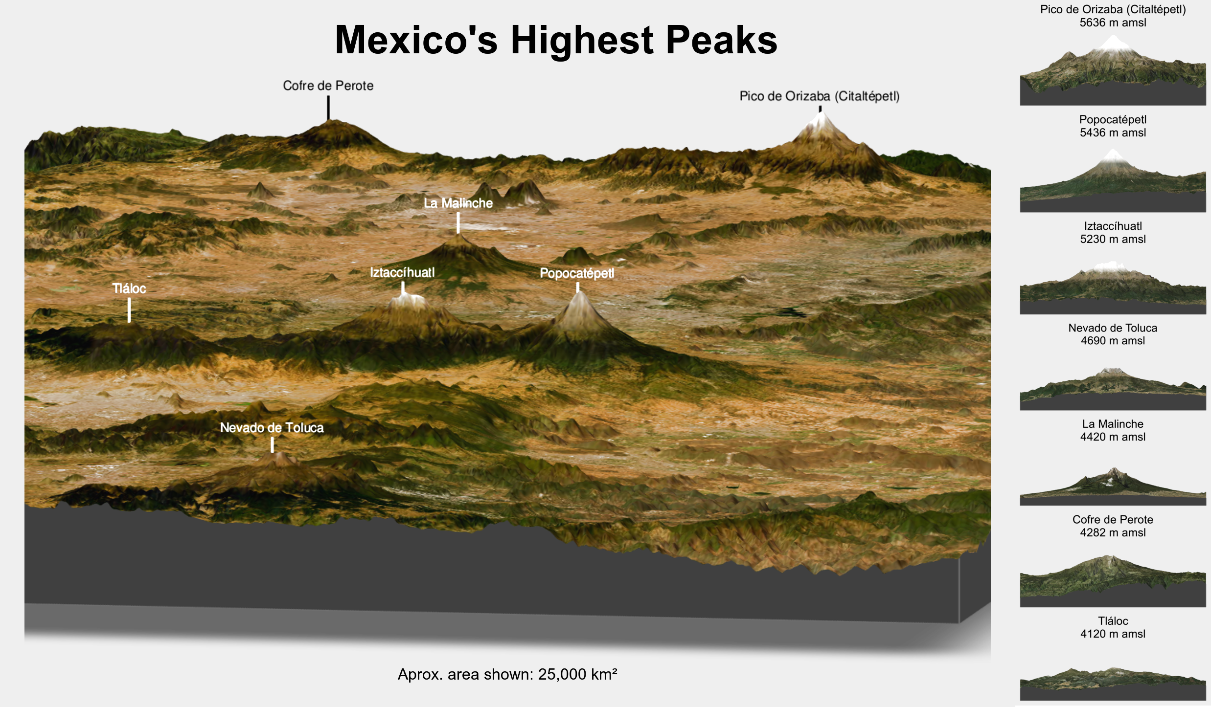 Mexico’s highest peaks.
In the final map, the tallest peaks can be appreciated with its labels, as well as a zoom-in to all of them individually (right-side panel). I like to think of the resulting image as a simple infography.