Beautiful plots in R using ggplot2

The purpose of this post is to show how to use the basic syntax of ggplot2, do some of the most common types of plots, as well as some customizations and facets. For this post we are going to use the iris dataset, as well as the skimr and cowplot packages. The first step consists of loading the desired packages, as well as the data and skimming over it. The first section will show some basic plots, while the next ones will show how to customize certain elements of the plots, like color, fill, facets and theme.

library(ggplot2)
library(skimr)
library(cowplot)

data(iris)
skim(iris)

Then we can start building our different plots.

Basic plots

Scatterplot

iris |>
  ggplot(aes(x = Sepal.Length, y = Sepal.Width)) +
  geom_point()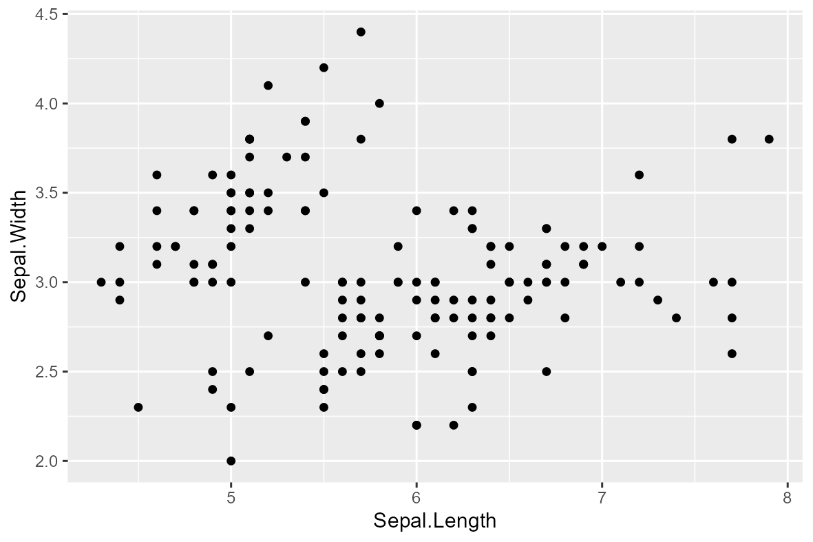

Scatterplot.

Line plot

iris |>
  ggplot(aes(x = Sepal.Length, y = Sepal.Width)) +
  geom_line()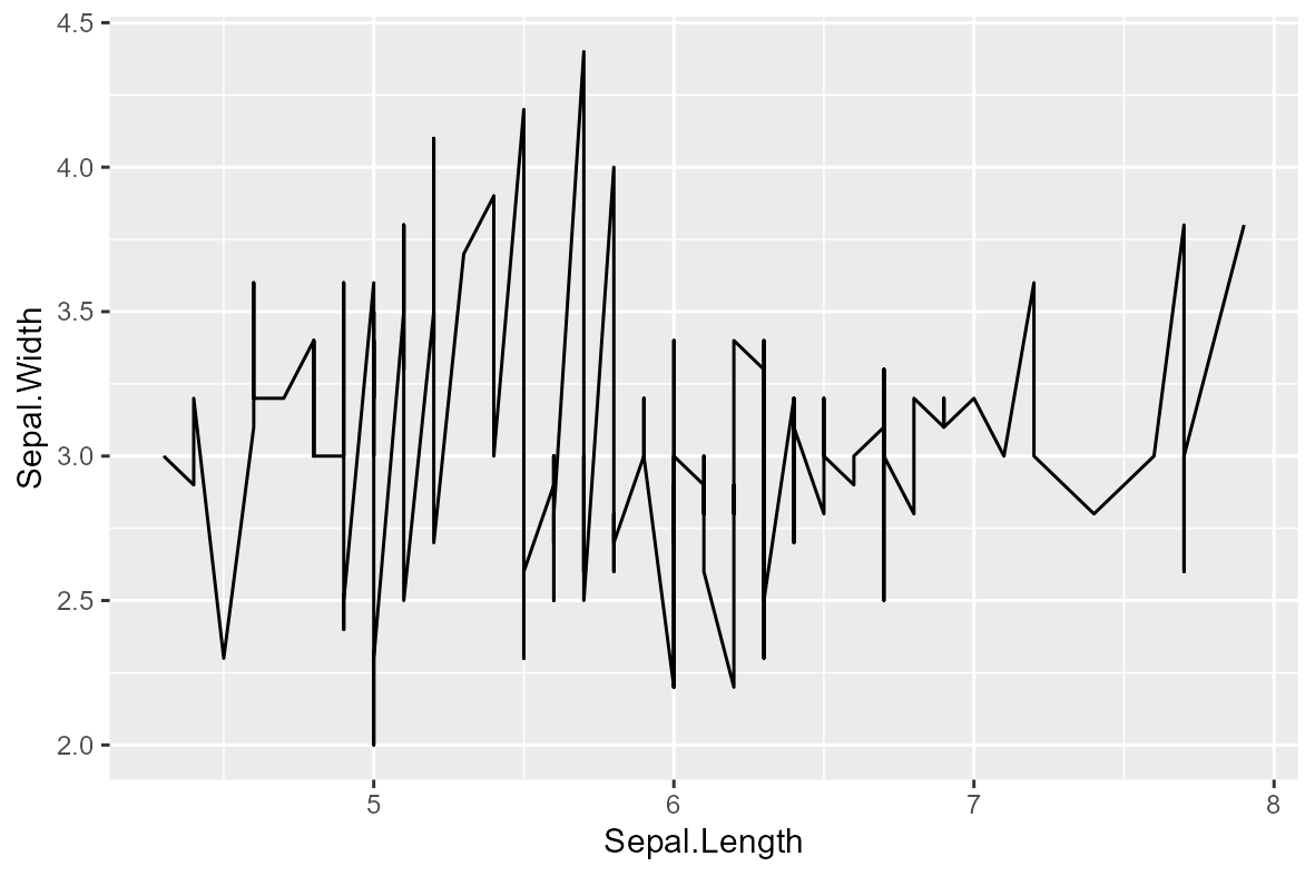

Line plot

Bar plot

iris |>
  ggplot(aes(x = Species)) +
  geom_bar()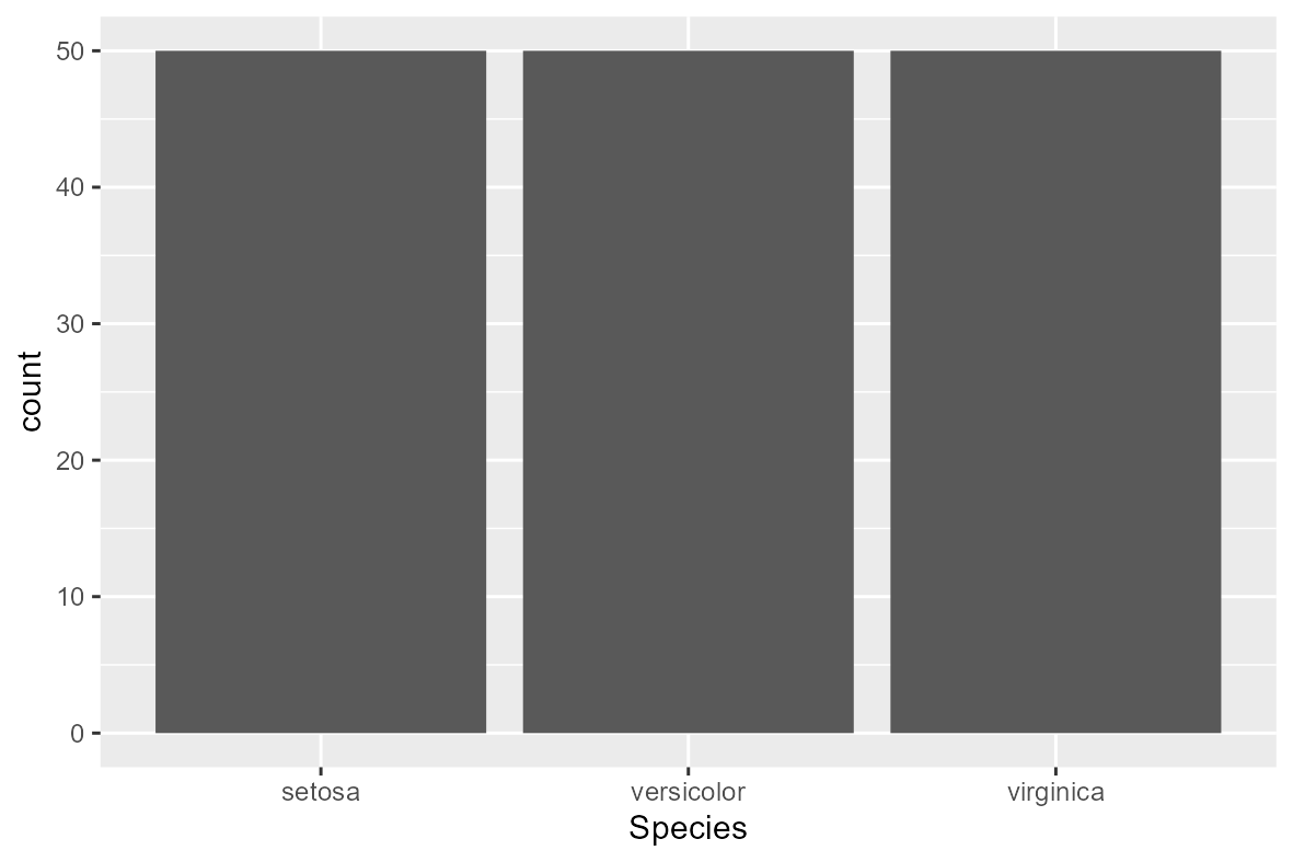

Bar plot.

Column plot

iris |>
  group_by(Species) |>
  summarise(meanSL = mean(Sepal.Length)) |>
  ggplot(aes(x = Species,
             y = meanSL)) +
  geom_col()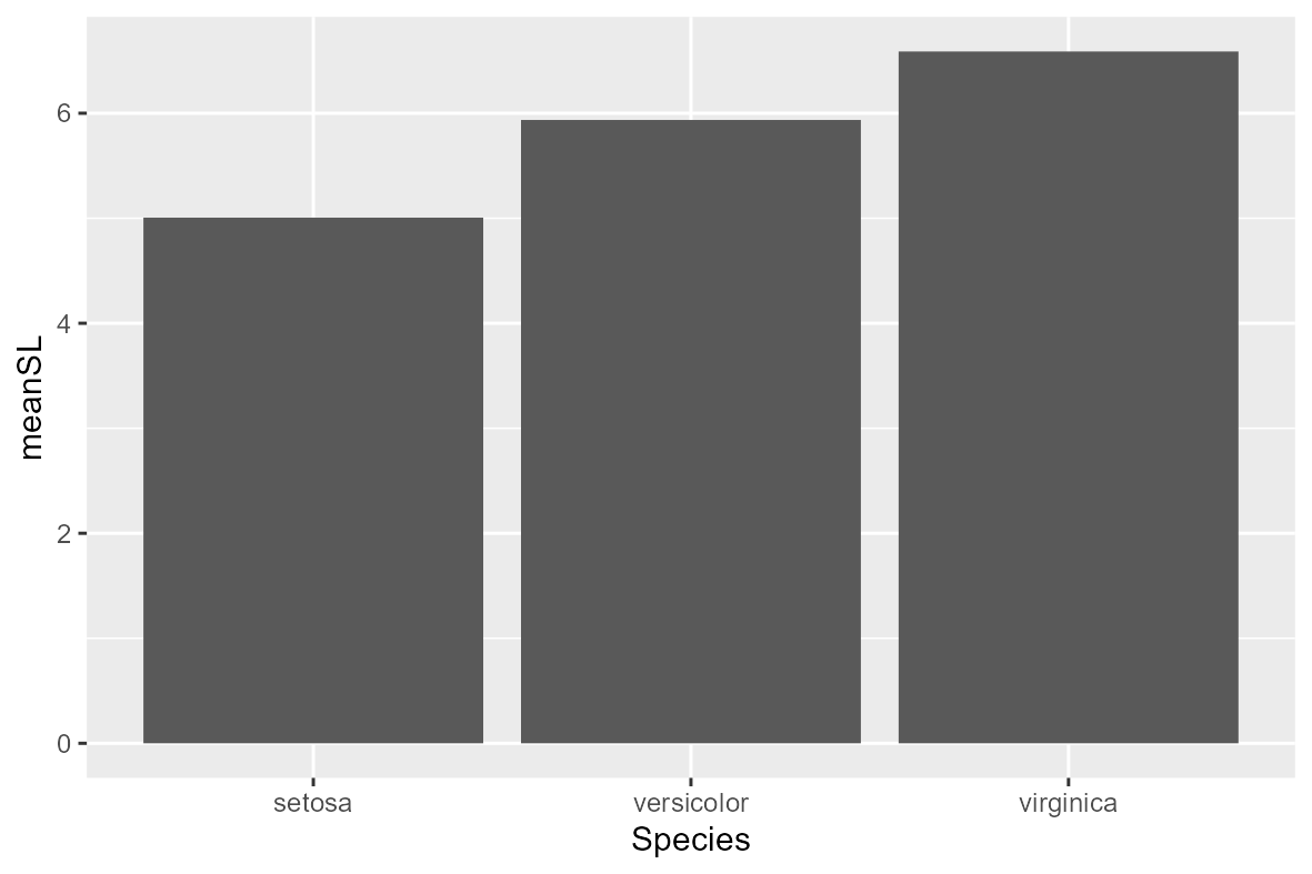

Column plot.

Box plot

iris |>
  ggplot(aes(x = Species,
             y = Sepal.Length)) +
  geom_boxplot()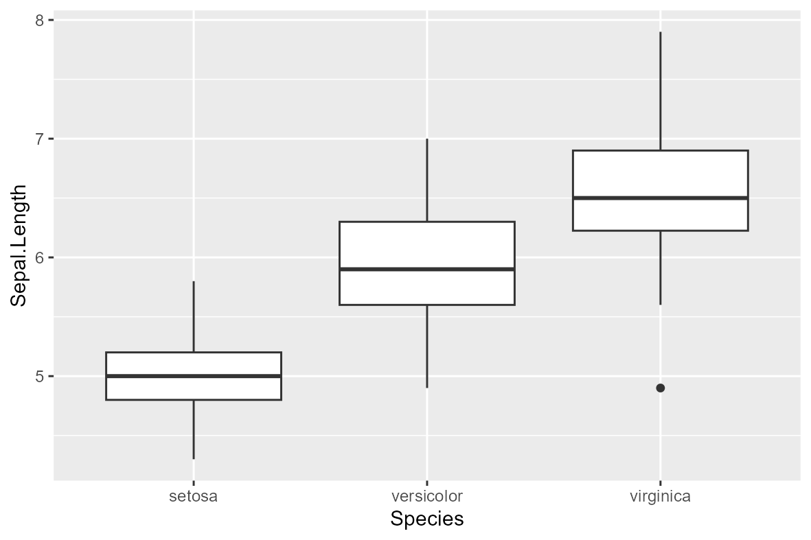

Boxplot.

Histogram plot

iris |>
ggplot(aes(x = Sepal.Length)) +
  geom_histogram()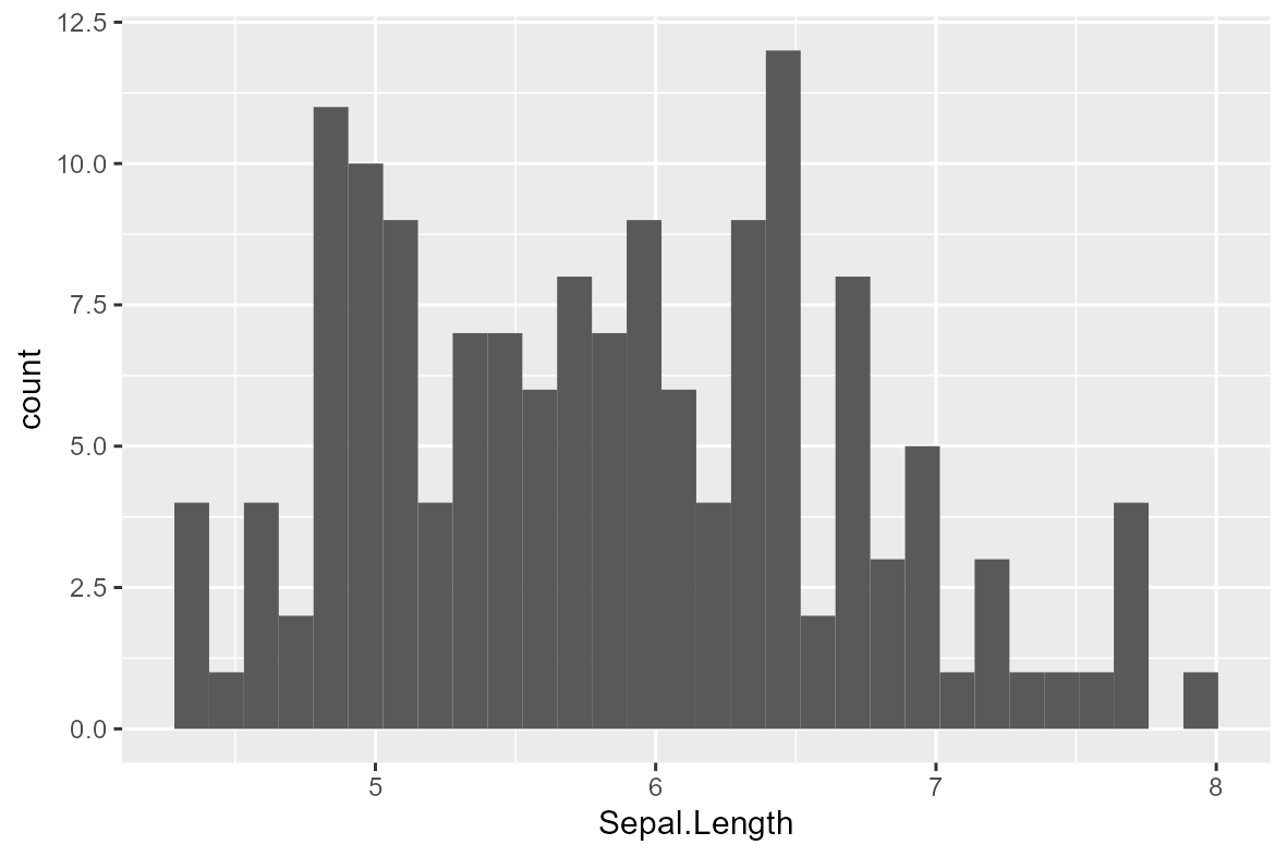

Histogram plot.

Adding colors

Color

iris |>
  ggplot(aes(x = Sepal.Length, 
             y = Sepal.Width,
             col = Species)) +
  geom_point()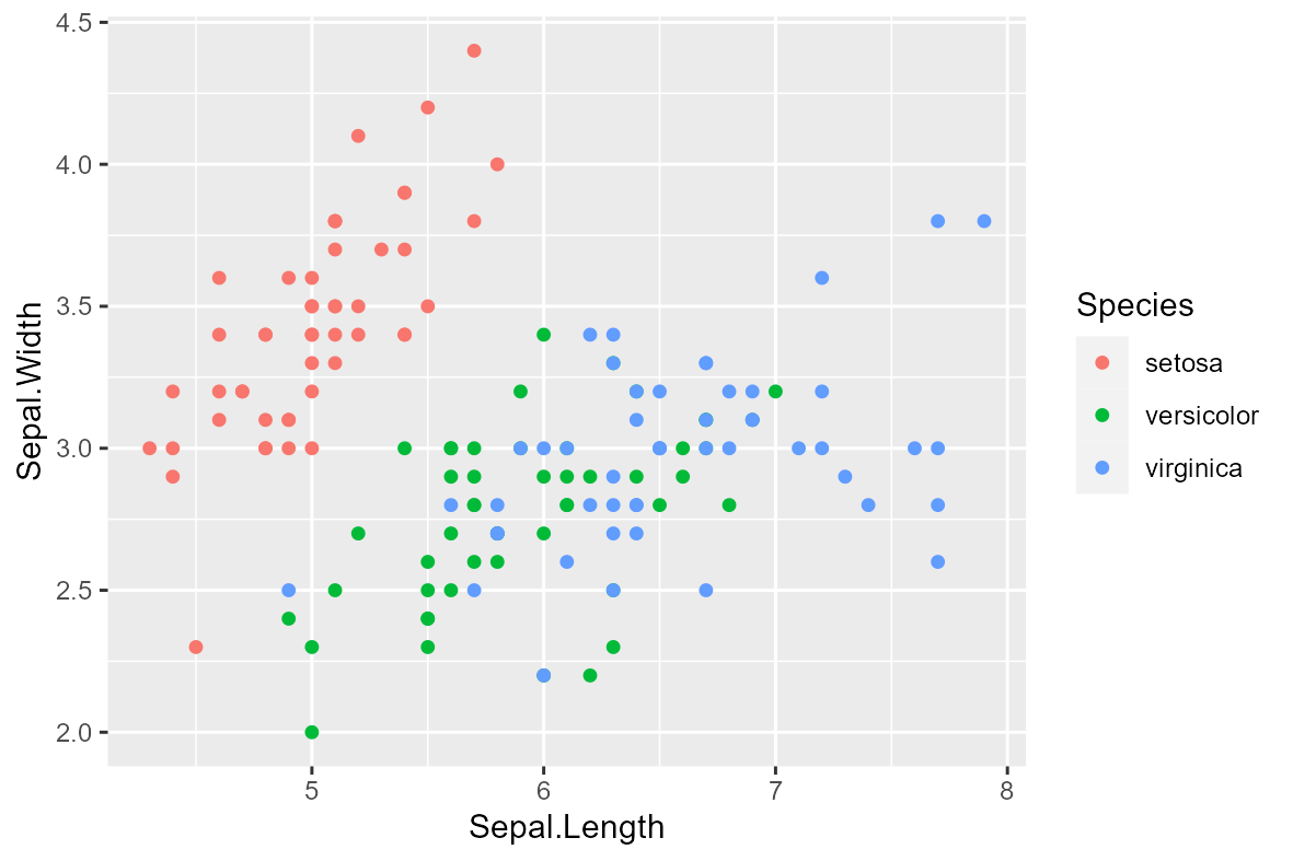

Scatterplot with colors by factor.

Fill

iris |>
  ggplot(aes(x = Species,
             fill = Species)) +
  geom_bar()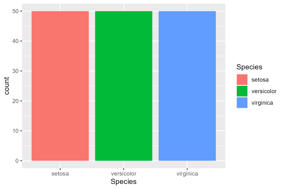

Barplot with fill by factor.

Customized colors

Manual colors

iris |>
  ggplot(aes(x = Sepal.Length, 
             y = Sepal.Width,
             col = Species)) +
  geom_point() +
  scale_colour_manual(values = c("forestgreen", "royalblue", "firebrick2"))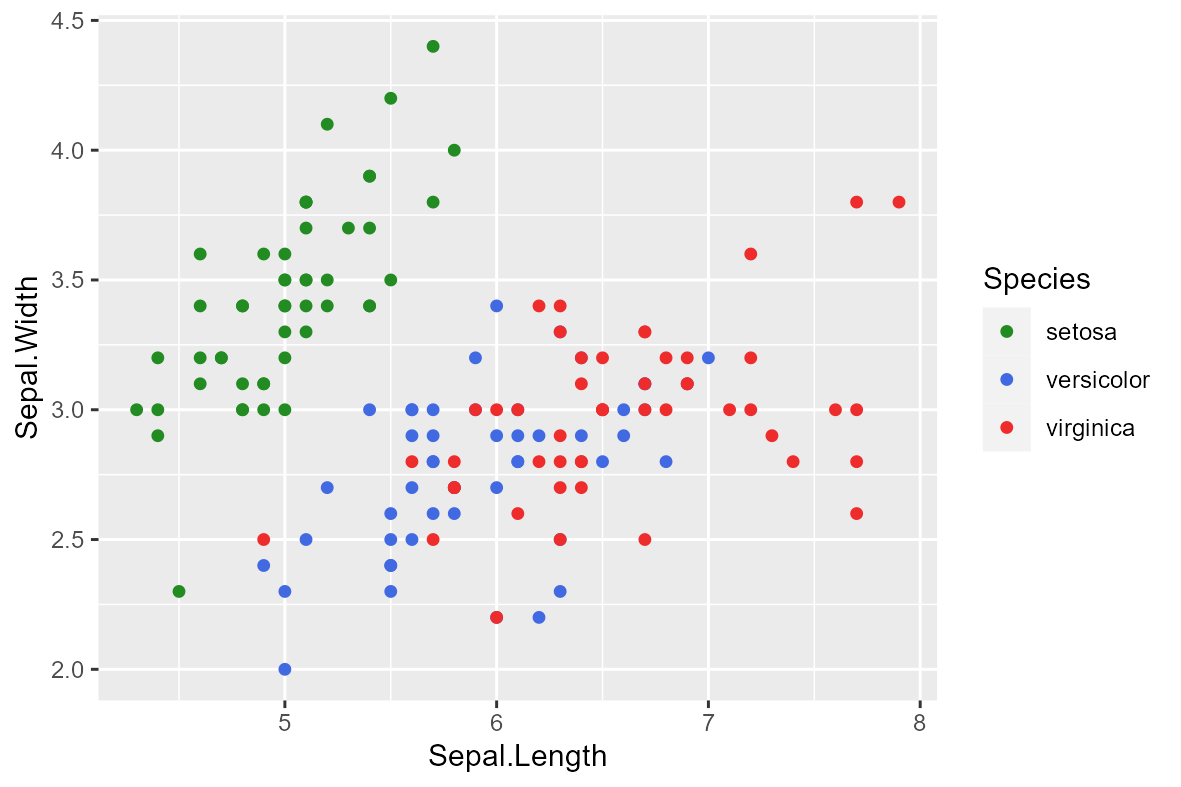

Scatterplot with manual colors by factor.

Rcolorbrewer

iris |>
  ggplot(aes(x = Sepal.Length, 
             y = Sepal.Width,
             col = Species)) +
  geom_point() +
  scale_colour_brewer(palette = "RdYlBu")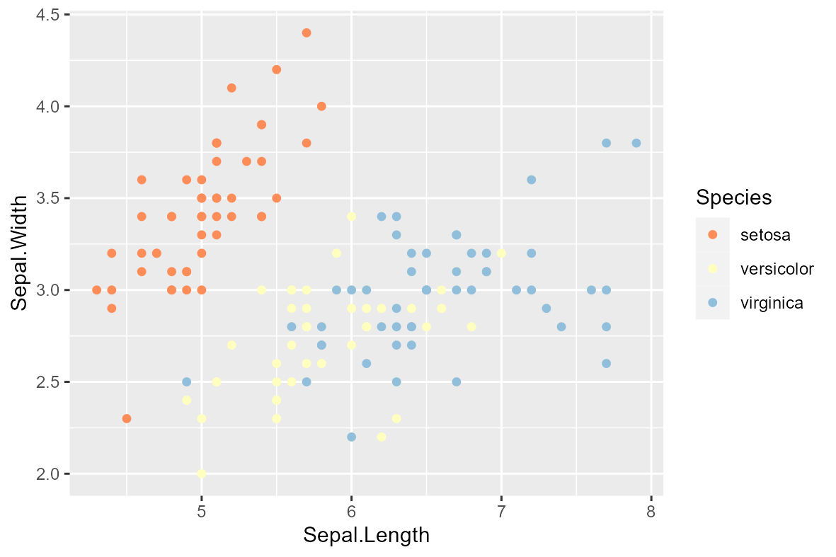

Scatterplots with colors set by RColorbrewer.

Axes

Axes

iris |>
  ggplot(aes(x = Sepal.Length, 
             y = Sepal.Width,
             col = Species)) +
  geom_point() +
  scale_y_continuous(breaks = seq(2, 4.5, 0.25),
                     limits = c(2, 4.5)) +
  scale_x_continuous(breaks = seq(4, 8, 0.5),
                     limits = c(4, 8))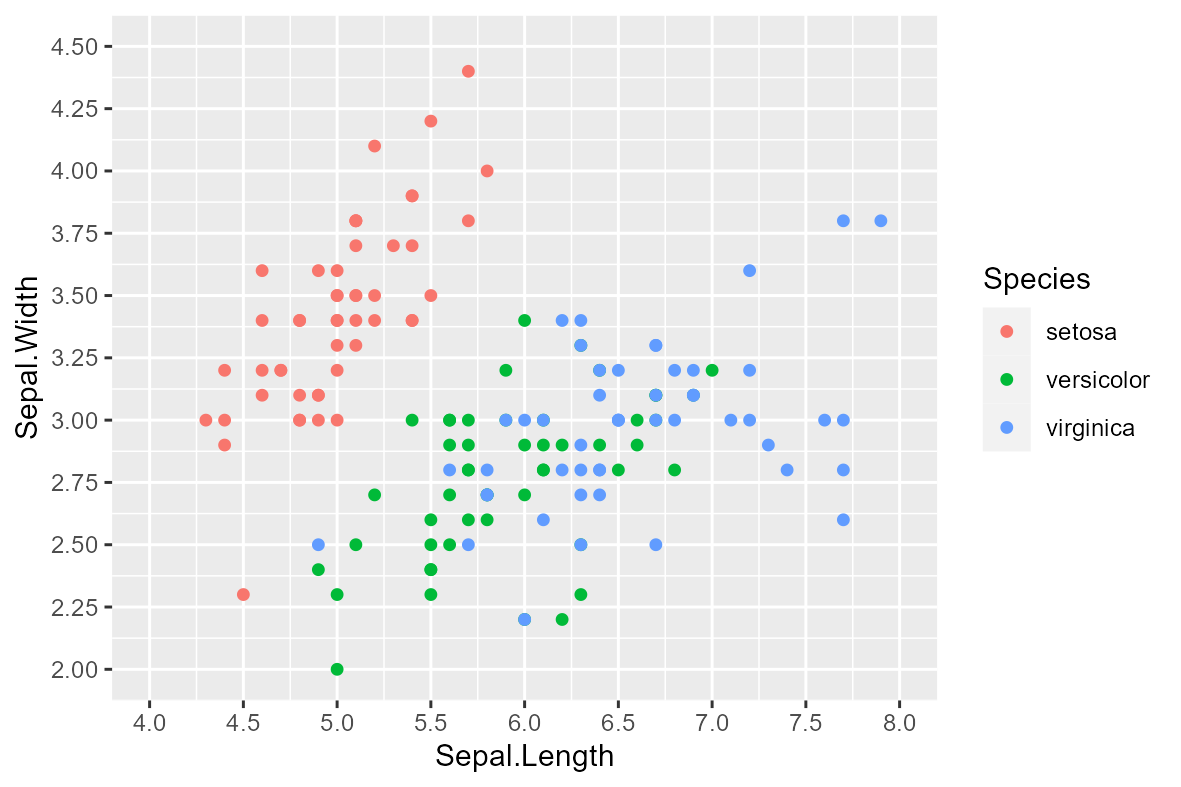

Scatterplot with customized axes.

Axes labels

iris |>
  ggplot(aes(x = Sepal.Length, 
             y = Sepal.Width,
             col = Species)) +
  geom_point() +
  labs(x = "Sepal length (cm)", 
       y = "Sepal width (cm)")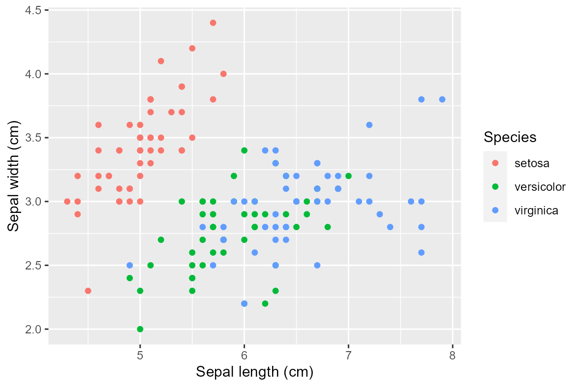

Scatterplot with customized axes labels.

Facets

Facet grid

iris |>
  ggplot(aes(x = Sepal.Length, 
             y = Sepal.Width,
             col = Species)) +
  geom_point() +
  facet_grid(~ Species)

Scatterplot with facets set as a grid.

Facet wrap

iris |>
  ggplot(aes(x = Sepal.Length, 
             y = Sepal.Width,
             col = Species)) +
  geom_point() +
  facet_grid(~ Species)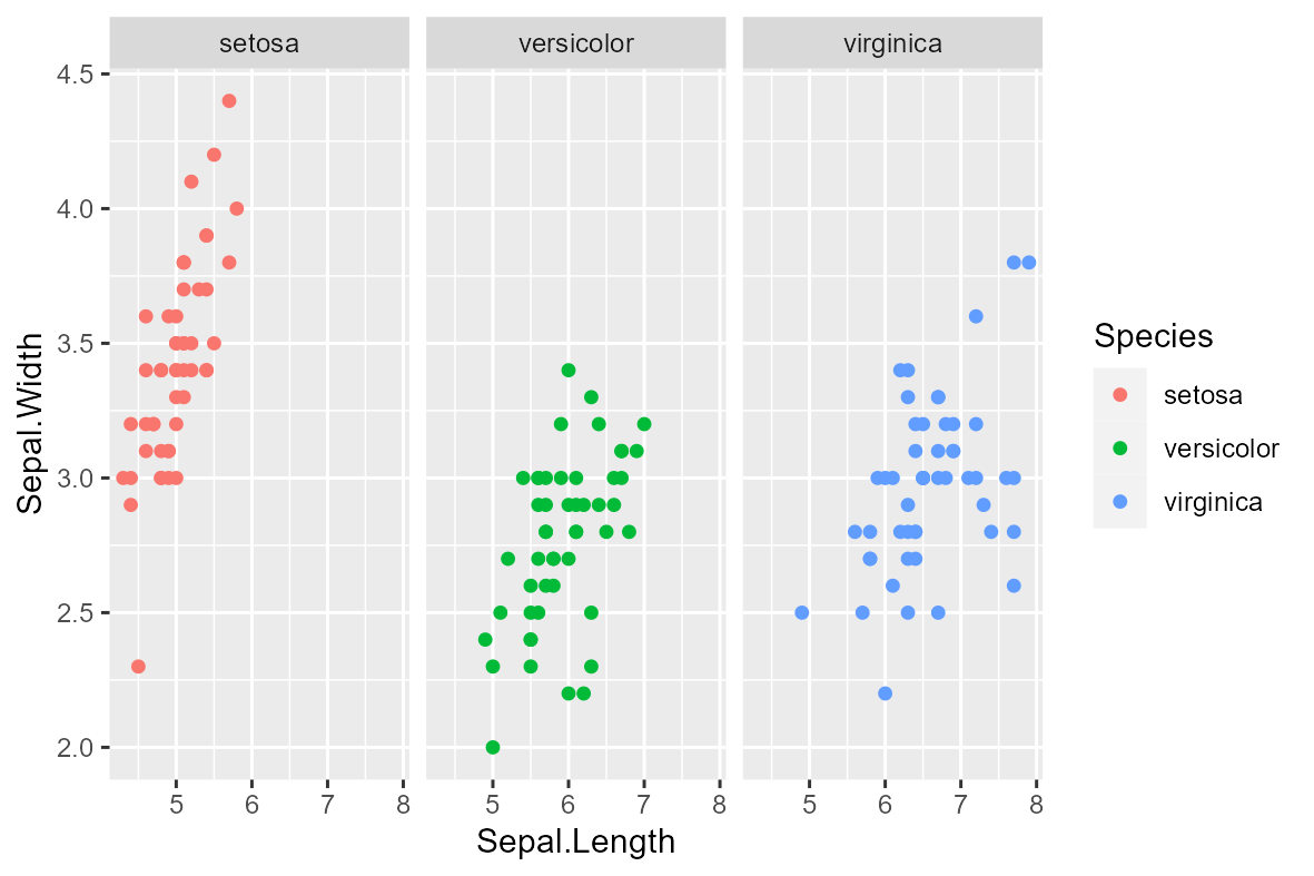

Scatterplot with facets set as a wrap (multiple factors will be accumulated by each panel).

Theme

Personalized theme

my_theme <- theme_bw() + 
  theme(plot.title=element_text(size=18,hjust = 0.5),
        text=element_text(size=24,colour="black"),
        axis.text.x = element_text(size=18,
                                   colour="black",
                                   angle = 90, 
                                   hjust = 1,
                                   vjust = 0.5),
        axis.text.y = element_text(size=18,
                                   colour="black",
                                   angle = 0, 
                                   vjust = 0.5,
                                   hjust = 1),
        axis.title = element_text(size=18,
                                  colour="black",
                                  face = "bold"), 
        axis.line = element_line(colour = "black"),
        legend.title = element_text(size=18),
        legend.text = element_text(size=18),
        axis.line.x =element_line(colour="black"),
        axis.line.y =element_line(colour="black"),
        panel.grid.major=element_blank(),
        panel.grid.minor=element_blank(),
        panel.border=element_blank(),
        panel.background=element_blank(),
        strip.background =element_rect(fill="gray90",
                                       colour = "black"),
        strip.text = element_text(size=18,
                                  colour="black",
                                  face = "bold"),
        plot.margin = unit(c(0.01,0.01,0.01,0.01), "cm"))

iris |>
  ggplot(aes(x = Sepal.Length, 
             y = Sepal.Width,
             col = Species)) +
  geom_point() +
  facet_wrap(~ Species) + 
  my_theme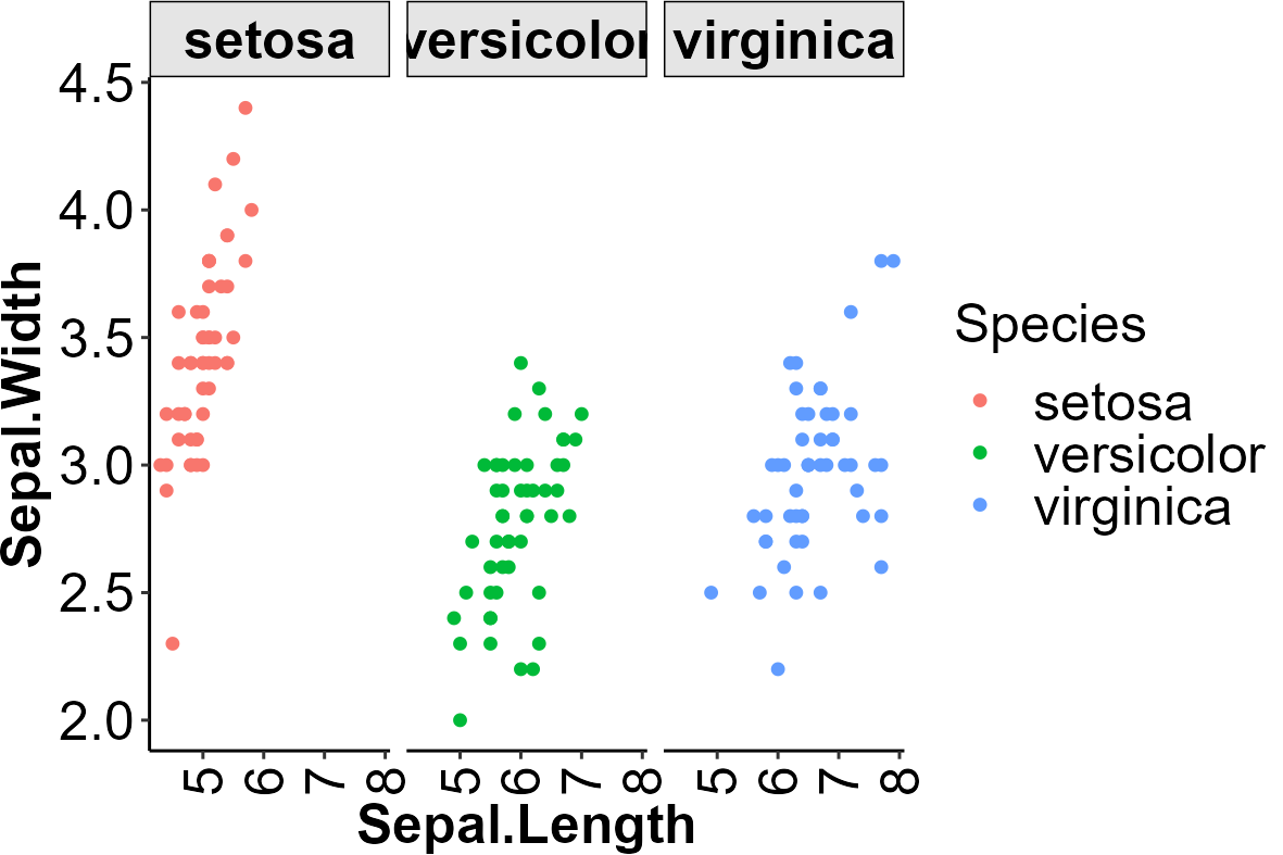

Scatterplot with facet wrap where several theme elements have been customized according to personal criteria.

Cowplot theme

iris |>
  ggplot(aes(x = Sepal.Length, 
             y = Sepal.Width,
             col = Species)) +
  geom_point() +
  facet_wrap(~ Species) + 
  theme_cowplot()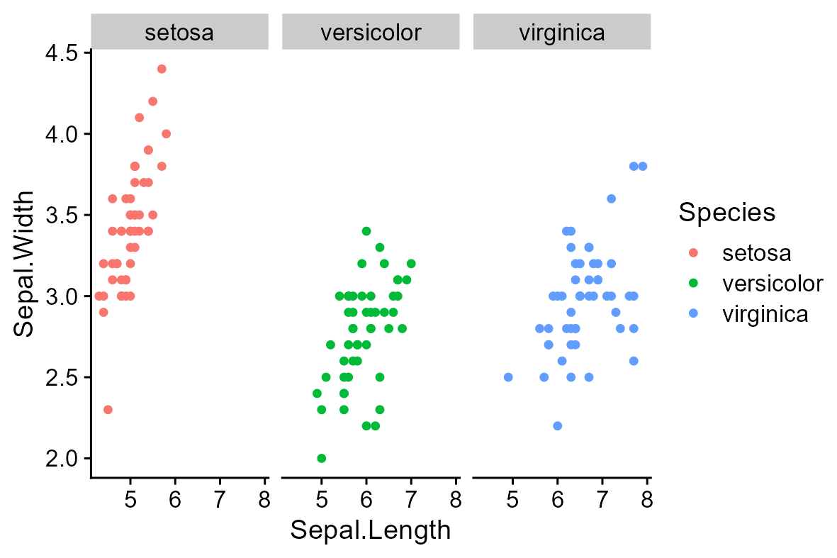

Scatterplot with facet wrap where several theme elements have been customized according to the cowplot theme.