Image texture in R

In this post I will show you how to calculate image texture in R. These textures have been used to model diversity and structural attributes of different forests with intermediate to very high R^2 values. Image textures are metrics that summarise the pixel’s tone variability in neighboring pixels using a particular window size. Thus, most of these metrics can be thought of variables sensing tone heterogeneity (or homogeneity) in space.

Image data

First we will create some dummy data just to make everything reproducible.

library(raster)

# Multispectral image
imgmul <- stack(list(raster(matrix(rnorm(25,0.3,0.1),nrow = 5)),
                     raster(matrix(rnorm(25,0.3,0.05),nrow = 5)),
                     raster(matrix(rnorm(25,0.2,0.05),nrow = 5)),
                     raster(matrix(rnorm(25,0.8,0.05),nrow = 5))))

# Get bands of interest, e.g., R and NIR
imgR<-imgmul[[3]]
imgNIR<-imgmul[[4]]

Here’s a preview of the dummy image: imgR.

Dummy image.

FOTO

Fourier transformed ordination is a method to calculate image texture that first uses the Fourier transform to summarise the spatial variation using harmonic waves (similar to sin and cos functions). Then, it applies a principal components analysis (PCA) over the previous data and usually works with the first three. Then, the PCA scores of the images are used as independent variables to model the forest attributes (usually measured in-field).

# Load library
library(foto)

# Set sizes of moving window size in pixels
vec_ventMS<-5 

# Calculate FOTO texture metrics
foto_resul <- foto(imgR, 
                   window_size = vec_ventMS, 
                   method="zones")

After doing these steps, you will get an object containing three entries: 1) zones, 2) radial spectra and 3) rgb. The first one contains the zones in which the image was divided to calculate the FOTO, the second one contains the radial spectra of the FOTO and finally, the third one contains the three first PCA components. The latter one, the PCA image, contains the information to model the forest’s attributes, so that image is the one that is going to be exported as raster.

# Make optional plots
# plot(PC.3)
# plotRGB(PC_stack,3,2,1,stretch="hist")
# plotRGB(PC_stack,3,2,1,scale=1)

# Write raster to disk  
writeRaster(foto_resul$rgb,
            paste0("R_DN_FOTO_nopad",vec_ventMS),
            type="INT2S",
            format="GTiff",
            overwrite=T)

Here’s a preview of the FOTO image.

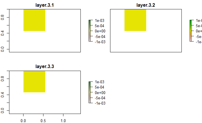FOTO images.

GLCM

Gray level co-ocurrence matrix texture is another apporach to calculate image texture. In this approach, the spatial heterogeneity is summarised by eight possible metrics: mean, variance, homogeneity, dissimilarity, contrast, entropy, asymptotic second moment and correlation. Each metric summarises a differnt aspect of image texture. The used approach will calculate these textures in the four possible directions (0°, 45°, 90° and 135 °) from a focal pixel. The other possible directions (180° - 360°) are mirrors of the previous directions. Then, the metrics calculated for each direction are averaged to obtain a single directionless metric.

# Load library
library(glcm)

# Set window size: horizontal and vertical dimensions
ventana_h<-9
ventana_v<-9

# Calculate glcm in the four possible directions, transforming the data into 64 levels of gray and using the previously set window
glcm_R<-glcm(imgR,shift=list(c(0,1), c(1,1), c(1,0), c(1,-1)),
             n_grey=64,
             window=c(ventana_v,ventana_h))

# Write to disk
# This image has 8 bands
writeRaster(glcm_R,
            paste0("R_DN_txts",ventana_h,"_",ventana_v),
            format="GTiff",
            datatype="FLT4S",
            overwrite=T)

Here’s a preview of the GLCM image.

GLCM images.