Making animations in R
This post will show you how to make animations in R.
The first step is to load the required packages. tidyverse is a package that contains other packages useful to wrangle and clean data, as well as to make plots, such as dplyr, tidyr and ggplot2. sf is a package that has several tools to work with vector data. gganimate is a package that will add animation to our plots.
library(tidyverse)
library(sf)
library(gganimate)
The second step is to read the data that is going to be used in the plot: the fires locations and week of occurence (fires.csv) and the region of interest shapefile (zm).
df <- read.csv("fires.csv",
               na.strings=c("", " ", "''"))

zm <- st_read("ROI.shp")
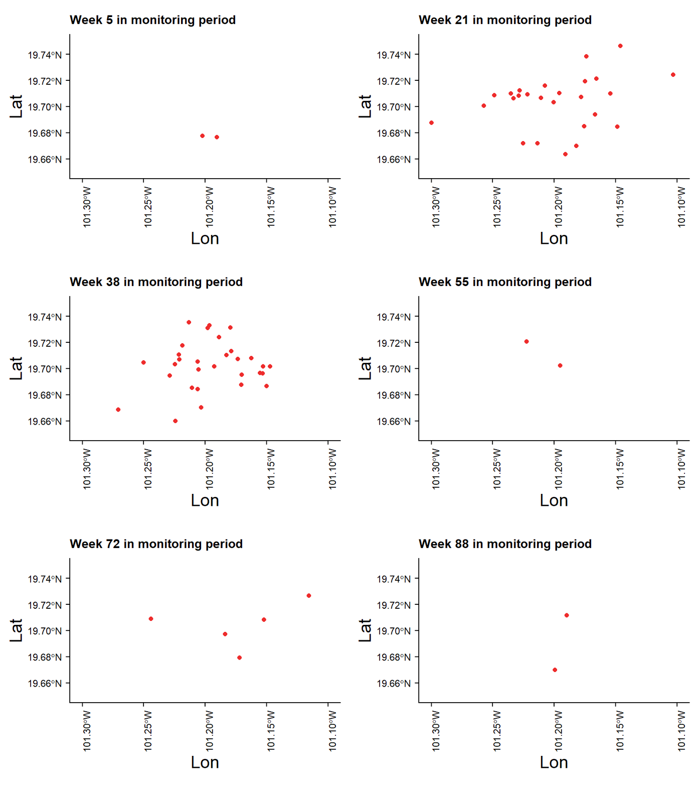
Next, let’s build the plot. The first part consists a fairly normal plot made with ggplot2, where we plot first the roi and then the fire occurence points and set other display specifics. After this part, we will set the title of the plot as a dynamic title which includes the frame_time of the animation rounded with zero decimals and paste this value along with a message. Then you need to specify the variable that represents the time steps. In this case, the time step variable is Semana, which means week in Spanish. Finally, we can add other chracteristics about the desired transition of the data between time steps, i.e., how the data enters into the dynamic plot (enter) and how it exits (exit). In this case, I chose both transitions as fade.
p1 <- ggplot (zm) +
  geom_sf(fill = "white") +
  geom_point(data = df,
             aes(x = lon,
                 y = lat),
             col = "firebrick2",
             size = 1.3,
             alpha = 1) +
  scale_x_continuous(limits = c(-101.3, -101.1)) +
  scale_y_continuous(limits = c(19.65, 19.75)) +
  cowplot::theme_cowplot() +
  theme(axis.text.x.bottom = element_text(size = 8,
                                          angle = 90),
        axis.text.y = element_text(size = 8),
        plot.title = element_text(size = 10)) +
  # Here comes the gganimate specific part
  labs(title = 'Week {round(frame_time,0)} in monitoring period',
       x = 'Lon', y = 'Lat') +
  transition_time(Semana) +
  enter_fade() +
  exit_fade()
If you wish to save the animation into a file, you can override the default size and resolution of the animation.
options(gganimate.dev_args = list(width = 800,
                                  height = 600,
                                  units = 'px',
                                  res=200))
Then, you need to animate the plot by defining the desired frames per second (fps) and number of frames (which can be set as the maximum value of the time steps in the data).
p1_anim <- animate(p1,
                   nframes = max(df$Semana),
                   fps=2)
Finally, save it as a gif.
anim_save("Plots/fires.gif",
          p1_anim)
And here’s a preview of the result.
