Diagrams in R
In this post I will show you how to create simple diagrams in R that can be useful for creating flowcharts and figures using the packages DiagrammeR. So the first thing is to load DiagrammeR package.
DiagrammeR package
library(DiagrammeR)This packages works with essentially two types of objects: nodes and edges. Nodes will represent the nodes in a diagram, which usually consist of geometric figures with text. In turn, edges correspond to connections among the nodes that will usually consist of arrows that represent the direction of the workflow. In this example, I will show you how to draw a diagram by adding each node and edge separately; however, for more experienced users it might be easier to use nodes and edge dataframes to define all the nodes and edges in a single data frame.
Example diagram
The first step is to create a graph, using the create_graph function. Then we will use a pipe |> to start creating each node, using add_node. Notice that each node can take the following arguments: label (text that will be shown) and font color of the node, shape of the node, color and fill color of the node. Additionally, you can set if the size of the figure should be set according to the label or a predefined height and width.
a_graph <- create_graph() |>
  # Set nodes
  add_node(label = "\nLandsat 5, 7, 8\nNDVI time\nseries (1994-\n2018)",
           node_aes = node_aes(
             shape = "cylinder",
             color = "#a4aebd",
             fillcolor = "#d9e8f8",
             fontcolor = "black",
             # fixedsize = T,
             height = 0.9,
             width = 1.1
           )) |>
  add_node(label = "BFAST\ncomponents\nextraction",
           node_aes = node_aes(
             shape = "box",
             color = "#be9c5c",
             fillcolor = "#fee5cc",
             fontcolor = "black",
             fixedsize = F
           )) |>
  add_node(label = "\n238 points\nTraining / Verification\nMagnitude\nGamma distribution",
           node_aes = node_aes(
             shape = "cylinder",
             color = "#8fa38a",
             fillcolor = "#d5e8d4",
             fontcolor = "black",
             # fixedsize = T,
             height = 0.9,
             width = 1.4
           )) |>
  add_node(label = "Visual interpretation\nusing Sentinel-2",
           node_aes = node_aes(
             shape = "rectangle",
             color = "#8e7571",
             fillcolor = "#f7cecc",
             fontcolor = "black",
             fixedsize = F
           )) |>
  add_node(label = "All-forest",
           node_aes = node_aes(
             shape = "rectangle",
             color = "#8b7e8f",
             fillcolor = "#e1d4e5",
             fontcolor = "black",
             fixedsize = F
           )) |>
  add_node(label = "TDF",
           node_aes = node_aes(
             shape = "rectangle",
             color = "#8b7e8f",
             fillcolor = "#e1d4e5",
             fontcolor = "black",
             fixedsize = F
           )) |>
  add_node(label = "TF",
           node_aes = node_aes(
             shape = "rectangle",
             color = "#8b7e8f",
             fillcolor = "#e1d4e5",
             fontcolor = "black",
             fixedsize = F
           )) |>
  add_node(label = "Models training\nand evaluation",
           node_aes = node_aes(
             shape = "oval",
             color = "#8b7e8f",
             fillcolor = "#e1d4e5",
             fontcolor = "black",
             fixedsize = F
           )) |>
  add_node(label = "Best model\nselection",
           node_aes = node_aes(
             shape = "rectangle",
             color = "#8b7e8f",
             fillcolor = "#e1d4e5",
             fontcolor = "black",
             fixedsize = F
           )) |>
  add_node(label = "Prediction on\nstudy site",
           node_aes = node_aes(
             shape = "rectangle",
             color = "#8b7e8f",
             fillcolor = "#e1d4e5",
             fontcolor = "black",
             fixedsize = F
           )) |>
  add_node(label = "\n624 points\n verification\nStratified random\ndistribution",
           node_aes = node_aes(
             shape = "cylinder",
             color = "#8fa38a",
             fillcolor = "#d5e8d4",
             fontcolor = "black",
             # fixedsize = T,
             height = 0.9,
             width = 1.1
           )) |>
  add_node(label = "Visual interpretation\nusing Sentinel-2",
           node_aes = node_aes(
             shape = "rectangle",
             color = "#8e7571",
             fillcolor = "#f7cecc",
             fontcolor = "black",
             fixedsize = F
           )) |>
  add_node(label = "Confusion matrix\ncalculation",
           node_aes = node_aes(
             shape = "rectangle",
             color = "#7c7b8c",
             fillcolor = "#d0cee3",
             fontcolor = "black",
             fixedsize = F
           )) |>
  add_node(label = "Class unbiased area\nestimate",
           node_aes = node_aes(
             shape = "rectangle",
             color = "#7c7b8c",
             fillcolor = "#d0cee3",
             fontcolor = "black",
             fixedsize = F
           ))
The second step is to define each node’s position. Notice that nodes are automatically numbered in the order they were created. Thus, node = 1 refers to the first node that was created using add_node. Each node position can be defined by its x and y coordinates.
a_graph <- a_graph |>
  # Set nodes position
  set_node_position(
    node = 1,
    x = 1, y = 6.5) |>
  set_node_position(
    node = 2,
    x = 2.45, y = 6.5) |>
  set_node_position(
    node = 3,
    x = 4, y = 6.5) |>
  set_node_position(
    node = 4,
    x = 3, y = 5) |>
  set_node_position(
    node = 5,
    x = 2, y = 4) |>
  set_node_position(
    node = 6,
    x = 3, y = 4) |>
  set_node_position(
    node = 7,
    x = 4, y = 4) |>
  set_node_position(
    node = 8,
    x = 3, y = 3)|>
  set_node_position(
    node = 9,
    x = 5, y = 3) |>
  set_node_position(
    node = 10,
    x = 5, y = 5) |>
  set_node_position(
    node = 11,
    x = 6.5, y = 6.5) |>
  set_node_position(
    node = 12,
    x = 6.5, y = 5) |>
  set_node_position(
    node = 13,
    x = 6.5, y = 4) |>
  set_node_position(
    node = 14,
    x = 6.5, y = 3)
Afterward, we will add the edges. In this step, we will use the same numbering of the nodes as in the previous step. Thus, node 1 will be the first created node, while node 2 will be the second. Inside the add_edge function we can set the width of the arrow, as well as its color.
a_graph <- a_graph |>
  # Add edges
  add_edge(from = 1, to = 2,
           edge_aes = edge_aes(
             penwidth = 1.5,
             color = "black")) |>
  add_edge(from = 2, to = 3,
           edge_aes = edge_aes(
             penwidth = 1.5,
             color = "black")) |>
  add_edge(from = 3, to = 4,
           edge_aes = edge_aes(
             penwidth = 1.5,
             color = "black")) |>
  add_edge(from = 4, to = 5,
           edge_aes = edge_aes(
             penwidth = 1.5,
             color = "black")) |>
  add_edge(from = 4, to = 6,
           edge_aes = edge_aes(
             penwidth = 1.5,
             color = "black")) |>
  add_edge(from = 4, to = 7,
           edge_aes = edge_aes(
             penwidth = 1.5,
             color = "black")) |>
  add_edge(from = 5, to = 8,
           edge_aes = edge_aes(
             penwidth = 1.5,
             color = "black")) |>
  add_edge(from = 6, to = 8,
           edge_aes = edge_aes(
             penwidth = 1.5,
             color = "black")) |>
  add_edge(from = 7, to = 8,
           edge_aes = edge_aes(
             penwidth = 1.5,
             color = "black")) |>
  add_edge(from = 8, to = 9,
           edge_aes = edge_aes(
             penwidth = 1.5,
             color = "black")) |>
  add_edge(from = 9, to = 10,
           edge_aes = edge_aes(
             penwidth = 1.5,
             color = "black")) |>
  add_edge(from = 2, to = 10,
           edge_aes = edge_aes(
             penwidth = 1.5,
             color = "black")) |>
  add_edge(from = 10, to = 11,
           edge_aes = edge_aes(
             penwidth = 1.5,
             color = "black")) |>
  add_edge(from = 11, to = 12,
           edge_aes = edge_aes(
             penwidth = 1.5,
             color = "black")) |>
  add_edge(from = 12, to = 13,
           edge_aes = edge_aes(
             penwidth = 1.5,
             color = "black")) |>
  add_edge(from = 13, to = 14,
           edge_aes = edge_aes(
             penwidth = 1.5,
             color = "black"))
Finally, we can render the graph.
render_graph(a_graph)The produced the diagram
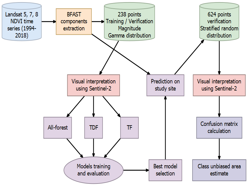 Flowchart of a BFAST + ML approach.
If you wish to export the diagram, you can use export_graph.
export_graph(a_graph,
             file_name = "Plots/flowchart.png",
             file_type = "png",
             width = 3600,
             height = 2400)