Making a map in R
In this post I will show you how to make a map with a reference map of the location of the study site. To achieve the desired map you will need to load several packages.
tmap is a package that lets you create plots from spatial information. sf is a package that has a lot of tools to work with vector information. tidyverse contains several packages such as tidyr, dplyr, ggplot2, which contain great functions to wrangle, plot and clean data. stars is a package that contains functions to work with raster information. RStoolbox is a package designed to work with remote sensing information, mainly rasters. cowplot is a package that easily lets you join several plots into a single one. Finally, gridExtra contains several functions designed to conver objects into graphical objects (grob) and arrange several plots into a single one.
library(tmap)
library(sf)
library(tidyverse)
library(stars)
library(RStoolbox)
library(cowplot)
library(gridExtra)
The next step is to load the vector and raster information used for the map. In this case, I will load a Sentinel-2 4 band image (R, G, B, NIR) and several shapes containing the world’s countries, Mexico and Guatemala polygons and a deforested areas shapefile. Finally, I am using st_make_valid to fix invalid geometries in the Guatemala and defor shapefiles.
masterIm <- read_stars("Sentinel-2_4B.tif")

world <- st_read("WorldWithoutMX.shp")
mx <- st_read("Mexico.shp")
gt <- st_read("Guatemala.shp")
gt <- st_make_valid(gt)

defor <- st_read("deforestation.shp")
defor <- st_make_valid(defor)
Next, I will transform the Sentinel-2 image into a stars object. Sometimes, very large rasters will be read as stars proxy objects, so you need to cast them into a stars object to apply several transformations. Finally, I define an RGB image from the Sentinel-2 one.
# Transform proxy object into stars
rgbIm <- st_as_stars(masterIm[,,,3:1])
rgbIm <- st_rgb(rgbIm,
                dimension = "band",
                maxColorValue = 6000,
                use_alpha = FALSE,
                probs = c(0.02, 0.98), #Probabilities for percent clip
                stretch = TRUE)
Additionally, I wish to create a bounding box polygon so the area covered by the image can be shown in the reference map.
box <- st_bbox(rgbIm)
box <- c(box[1]+0.2,box[2]+0.2,box[3]-0.2,box[4]-0.2)
Afterward, the main map is created. Each element will be added to the map by using the tm_shape functions to indicate the source data to plot, followed by a tm_* function indicating the type of object, i.e., raster or filled polygons (tm_fill). Then, the graticules of the map are added using tm_graticules and the scale bar, using tm_scale_bar. Finally, you can make further customisations to the default theme, using tm_layout. Finally, the map is converted to a graphical object (grob) using tmap_grob()
# Normal map
plot_im <- tm_shape(rgbIm,
                    bbox = box) +
            tm_raster() +
            tm_shape(gt) +
            tm_fill(col = "gray90",
                    alpha = 0.95) +
            tm_shape(defor) +
            tm_fill(col = "finid",
                    border.col = "transparent",
                    lwd = 2,
                    legend.show = F,
                    palette = c("1" = "firebrick2", "2" = "yellow2", "3" = "royalblue")) +
            tm_graticules(n.x = 5,
                          n.y = 5,
                          labels.show = T,
                          labels.format = list(fun = function(x){
                            degs <- floor(x)
                            decs <- (x %% 1)
                            mins <- floor(decs*60)
                            paste0(degs, "°", mins, "\'")}),
                          labels.rot = c(90,0),
                          labels.cardinal = T,
                          ticks = T,
                          lines = F) +
            tm_layout(legend.only = F,
                      legend.outside = T,
                      attr.outside = F,
                      legend.outside.position = "right",
                      # legend.position = c(0.1,0.7),
                      # attr.position = c(1.2, -0.05),
                      between.margin = c(0),
                      outer.margins = c(0.1),
                      inner.margins = c(0.1),
                      fontface = "bold",
                      fontfamily = "sans")  +
            tm_scale_bar(breaks = seq(0,10,5),
                         position = c(0.35, 0.001),
                         text.size = 0.6,
                         text.color = "white",
                         color.dark = "gray10",
                         color.light = "white",
                         just = "right",
                         bg.color = "gray90",
                         bg.alpha = 0.2)

plot_im <- tmap_grob(plot_im)
Once the main map has been created, you will need to create the legend of the map. So you can place it in the desired position outside the main map. To do this, you need to draw a map containing the information shown in the legend. Notice that the tm_layout enables a legend.only option to just create an object containing the legend. Then, the legend is converted to a grob.
legend_im <- tm_shape(defor) +
  tm_fill(col = "finid",
          border.col = "transparent",
          lwd = 2,
          title = "Type of observation",
          labels = c("Old-growth forest loss",
                     "Secondary forest or plantation loss",
                     "Loss in the next year"),
          palette = c("1" = "firebrick2", "2" = "yellow2", "3" = "royalblue")) +
  tm_layout(legend.only = T,
            legend.outside = T,
            legend.outside.size = 0.5,
            attr.outside = F,
            legend.outside.position = "right",
            # legend.position = c(0.1,0.7),
            # attr.position = c(1.2, -0.05),
            between.margin = c(0),
            outer.margins = c(0.1),
            inner.margins = c(0.1))

legend_im <- tmap_grob(legend_im)
Then, you will need the bounding box as a spatial feature, so it can be added to the map. Additionally, you need to create an object containing the bounding box to be drawn on the reference map (mx_box).
box_shape <- st_bbox(rgbIm) |>
              st_as_sfc()

mx_box <- st_bbox(mx)
The next step is to create the reference or inset map that will show the context of the study area. In this case, this map will show neighboring countries of Mexico, as well as the study site location. Similar to the first map, the result is converted to a grob.
inset_im <- tm_shape(world,
                     bbox = mx_box)+
  tm_polygons(col = "gray90") +
  tm_shape(mx) +
  tm_polygons(col = "gray75") +
  tm_text("COUNTRY", size = 0.5) +
  tm_shape(box_shape) +
  tm_borders(col = "firebrick2",
             lwd = 2)

inset_im <- tmap_grob(inset_im)
To have better control of the position of every element in the map, you will need to create an empty plot as base plot, so afterward, all the other elements will be placed over this empty plot. Additionally, you need to create an additional grob with text that shows the datum of the showed data.
# Create empty plot as base
p1 <- ggplot() +
  geom_blank() +
  theme_void()

texto <- text_grob(label = "WGS 84",
                   size = 8)
Next, you need to draw all the elements on the empty plot and set its x and y positions, as well as width and height values. All these values are limited to a 0-1 range. However, negative values can be used to reduce the size of certain margins and obtain the desired position.
exp_plot <- ggdraw(p1) +
  draw_plot(plot_im,
            x = -0.17,
            y = -0.14,
            hjust = 0,
            vjust = 0,
            width = 1,
            height = 1.2) +
  draw_plot(inset_im,
          x = 0.75,
          y = 0.72,
          hjust = 0,
          vjust = 0,
          width = 0.2,
          height = 0.2) +
  draw_plot(legend_im,
            x = 0.55,
            y = -0.12,
            hjust = 0,
            vjust = 0,
            width = 0.5,
            height = 0.8) +
  draw_plot(texto,
            x = 0.73,
            y = 0.1,
            hjust = 0,
            vjust = 0,
            width = 0.2,
            height = 0.2)
Finally, you can export the resulting map using save_plot.
save_plot(exp_plot,
          # asp = 1.5,
          base_width = 20,
          base_height = 15,
          units = "cm",
          dpi = 300,
          filename = "Map/Map1.jpeg")
Here is the resulting map.
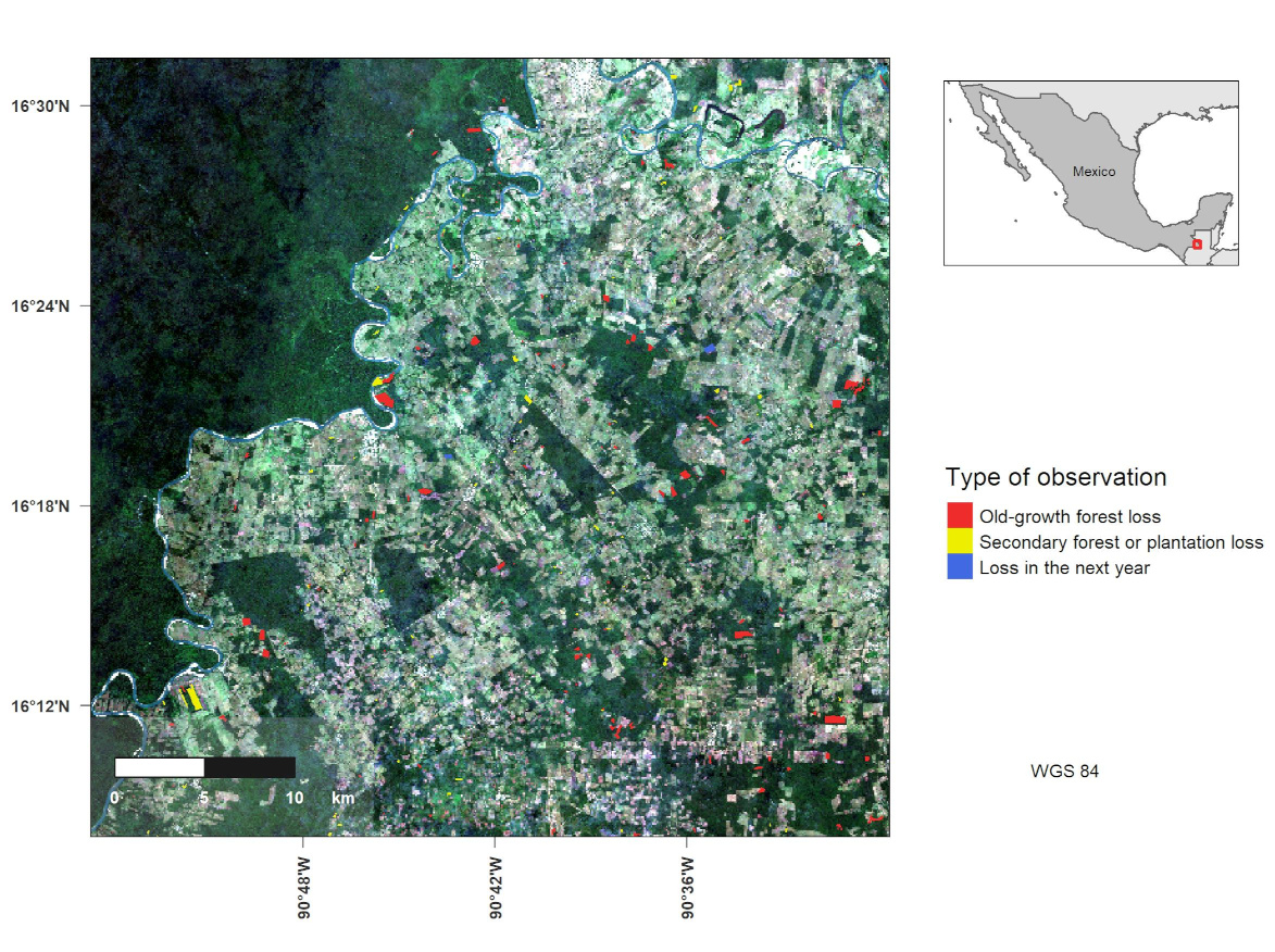 Map of the study site with an inset map.