Rasters and vectors with terra
This post shows a simple example of how to work with rasters and vectors using the terra package. Terra replaces the older raster package, since terra is usually faster to use.
library(tibble)
library(terra)
library(dplyr)
Then create some objects to work with and plot them.
im1 <- rast(matrix(1:9, nrow = 3),
crs = "EPSG:4326",
extent = c(-103,-100,19,22))
pts1 <- vect(data.frame(lon = c(-102.5, -102.5, -100.5, -100.5),
lat = c(19.5, 21.5, 21.5, 19.5)),
geom = c("lon", "lat"),
crs = "EPSG:4326")
poly1 <- vect("POLYGON ((-102.5 19.5, -102.5 21.5, -100.5 21.5, -100.5 19.5, -102.5 19.5))",
crs = "EPSG:4326")
plot(im1)
plot(pts1, add = T)
plot(poly1, add = T)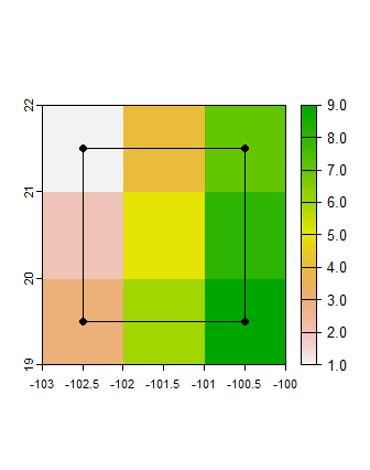 Data.
Data.
Vector operations
Buffer
poly2 <- buffer(poly1, width = 10000, capstyle = "square")
plot(poly2)
plot(poly1, add = T)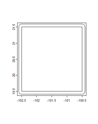 Buffer.
Intersection
poly3 <- intersect(poly2, poly1)
plot(poly3[[1]])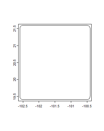 Intersection.
Raster operations
Mask values
im2 <- im1
im2[im2>=5] <- NA
plot(im2)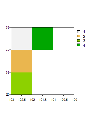 Masked raster.
Operations over all cells
# Stack same image
im3 <- c(im1, im1)

im4 <- app(im3, fun = "sum")
plot(im4)
Sum of both bands.
Global operations
global(im1, fun = "mean")
      mean
lyr.1    5
Focal operations
im5 <- focal(im1, w = 3, fun = "max")
plot(im5)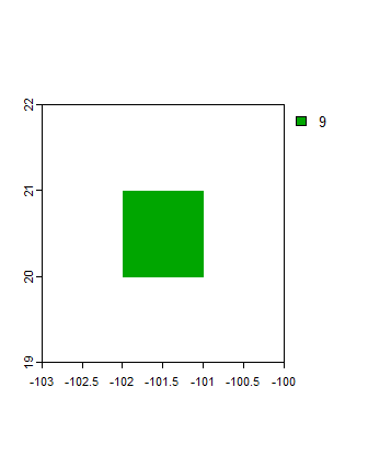 Focal max.
Raster vector operations
Crop
im1_c <- crop(im1, poly1)
plot(im1_c)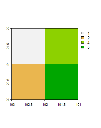 Cropped images.
Mask
im2_c <- mask(im1, poly1)
plot(im2_c)
Masked image (seems nothing happened due to overlap between raster and polygon).
Extract values
Manual colors
expts <- extract(im1, pts1)

# Get x and y coordinates and value
geom(pts1) |>
  as_tibble() |>
  select(x, y) |>
  mutate(value = expts|>pull(lyr.1))

# A tibble: 4 × 3
      x     y value
  <dbl> <dbl> <int>
1 -102.  19.5     3
2 -102.  21.5     1
3 -100.  21.5     7
4 -100.  19.5     9