RGB Shaded relief maps in R

In this post I will show you how to make an RGB composite with shaded relief using rayshader, elevatr, maptiles,sf, terra and magick packages. First load the libraries we are going to use.

library(elevatr)
library(maptiles)
library(sf)
library(terra)
library(rayshader)
library(magick)

Then, read the roi polygon file and use it to obtain the RGB tiles and DEM data.

# Get polygon of roi
# Can be downloaded from: https://github.com/JonathanVSV/Ppage2/tree/master/assets/data
poly <- st_read("MX_inegi.gpkg")
# Get RGB mosaic
rgb <- get_tiles(poly,
                 provider = "Esri.WorldImagery",
                 cachedir = "cache",
                 crop = T,
                 zoom = 6)
# Get elevation data using elevatr
dem <- get_elev_raster(poly,
                      prj = "EPSG:4326",
                      src = "aws",
                      z = 6,
                      neg_to_na = FALSE)

Then, mask the images using the roi’s polygon and crop the dem to the extent of the RGB.

# Mask areas according to polygon
rgb <- mask(rgb, poly)
dem <- mask(dem, poly)

# Crop dem extent to rgb
dem <- crop(rast(dem), rgb)

Afterward, transform the RGB into an array and the dem into a matrix.

# Restack
# And convert it to a matrix:
dem_mat <-  raster_to_matrix(dem)
rgb_mat <- as.array(rgb)

Make a hillshade using the dem (as matrix). Transform it to rast again, set its extent and mask with the roi’s polygon.

# Make hillshade
hillshade <- dem_mat %>%
  sphere_shade(sunangle = 315,
               texture = 'bw',
               zscale = 250,
               colorintensity = 0.5)

# Convert back to rast
hillshade <- rast(hillshade)

# Add extent from rgb and mask
ext(hillshade) <- ext(rgb)
hillshade <- mask(hillshade, poly)

Then export the two images in a single png, setting some transparency in the second image so the hillshade can be appreciated under the RGB composite. In this case, you need to create a folder named “Plots” outside R in your working directory or use dir.create("Plots") inside R, so you can export the file in the exact same location as in the example. Other alternative, might be to delete the folder part (i.e., “Plots/”)and just export it directly in the working directory.

# Export to png
png("Plots/Mexico_hillshade.png",
    width = 20,
    height = 15,
    units = "cm",
    res = 300)

# Plot hillshade
plotRGB(hillshade, 
        stretch = "hist",
        smooth = T,
        # completely opaque
        alpha = 255,
        add = F,
        maxcell=Inf, 
        # Make zoom to the bounding box of the roi
        xlim = c(st_bbox(poly)[[1]]-0.05,st_bbox(poly)[[3]]+0.1),
        ylim = c(st_bbox(poly)[[2]],st_bbox(poly)[[4]]))

# Plot RGB composite
plotRGB(rgb, 
        stretch = "lin",
        smooth = T,
        # Partially transparent
        alpha = 180,
        # Add to previous plot
        add = T,
        maxcell=Inf) 

dev.off()

Once you obtain the png, you will see that the colors of the image are somewhat pale. Thus, you can use magick to increase the saturation of the colors, increase the contrast and write the image into another png.

# Final enhancements
# Read image
im1 <- image_read("Plots/Mexico_hillshade.png")
# Add color saturation
im2 <- image_modulate(im1, 
                      brightness = 100, 
                      saturation = 200, 
                      hue = 100)
# Increase contrast
im2 <- image_contrast(im2, sharpen = 2)
# Write image
image_write(im2, 
            path = "Plots/Mexico_hillshade_final.png", 
            format = "png")

The result:

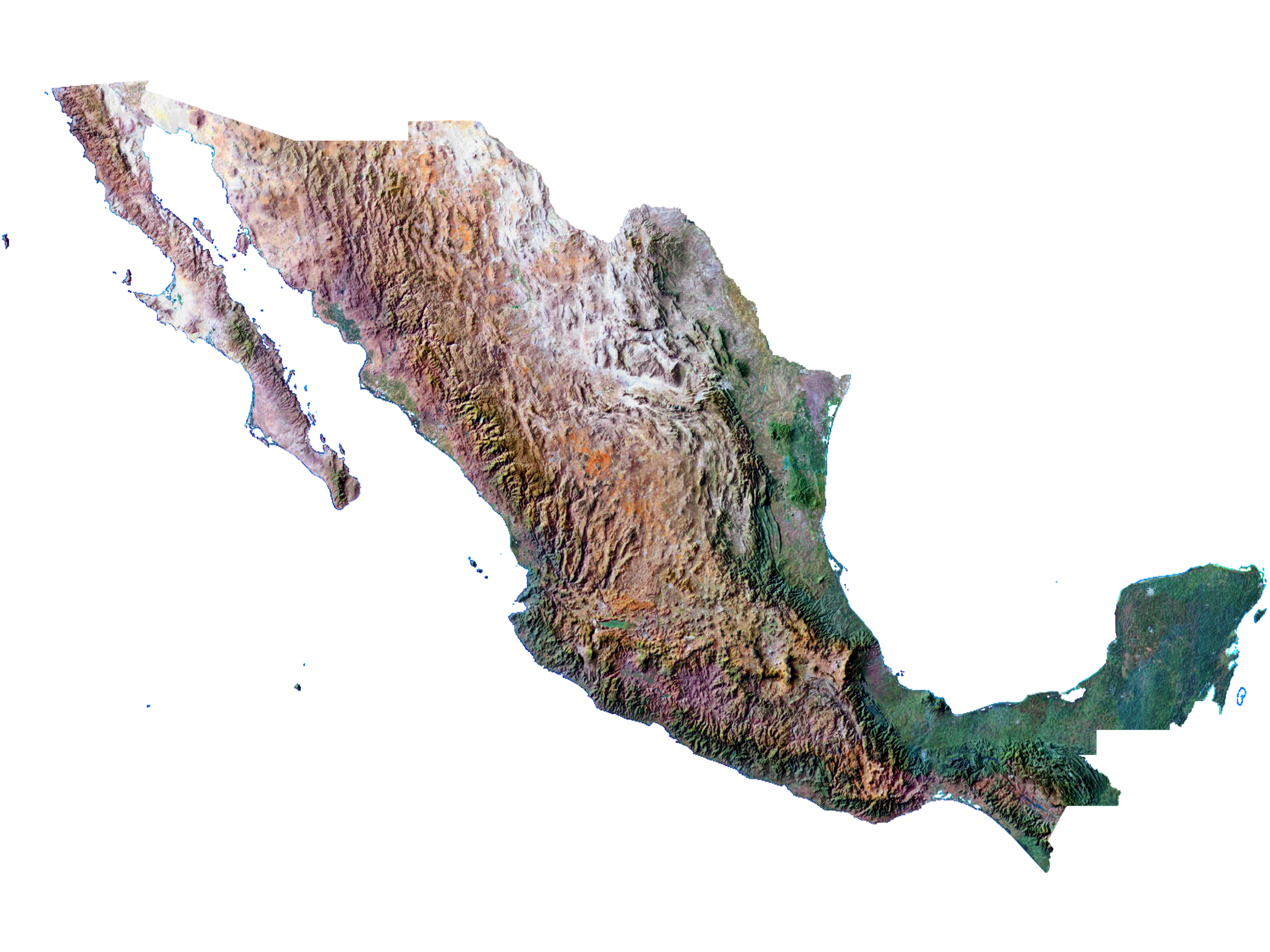RGB shaded relief map of Mexico.

If you are familiar with the surrounding of Morelia, Michoacán, Mexico, you will immediatly recognize Patzcuaro and Cuitzeo lakes, as well as some hills, such as the Quinceo.