Shaded relief maps in R
This is a follow up of the series of experiments I have been working with rayshader. In this post, I will focus on making a shaded relief map using different colors to represent different altitudes. Also, in this post I will show you how to visualize the shaded relief map with a given projection and add some labels to the final map.
library(elevatr)
library(sf)
library(terra)
library(rayshader)
library(magick)
Define some variables: name of the polygon to save the files, the name used to add a label at the end, the CRS to project the visualization of the map, and some variables to render the shaded relief and final labels. In this case, I had to use PROJ notation to define the projection to which I wanted the map to be projected to; although, nowadays this notation is discouraged in favor of WKT2 notation or EPSG or ESRI codes.
name_poly <- "Mexico"
name_legend <- "Mexico"
# Had to use proj4, although it is not prefered over epsg codes
# However there was no epsg:6361
newProj <- "+proj=lcc +lat_0=12 +lon_0=-102 +lat_1=17.5 +lat_2=29.5 +x_0=2500000 +y_0=0"
sunangle <- 315
# Lower value more z exaggeration
zscale <- 20
zoom_val <- 6
sunaltitude <- 30
font <- "sans"
font_color <- "#01611F"
Then, read the roi polygon file and use it to obtain the DEM data.
# Get polygon of roi
# Can be downloaded from: https://github.com/JonathanVSV/Ppage2/tree/master/assets/data
poly <- st_read("MX_inegi.gpkg")
# Get RGB mosaic
# Get elevation data using elevatr
dem <- get_elev_raster(poly,
                      prj = "EPSG:4326",
                      src = "aws",
                      z = zoom_val,
                      neg_to_na = FALSE)
Then, extract the bounding box coordinates of the polygon to add them in the add as a notation in the final image. Do some adjustments such as round to two decimals and add N and W letters.
box_coords <- st_bbox(poly)
coords_df <- data.frame(c1 = paste0(abs(round(box_coords[2],2)), "° N, ",
                                    abs(round(box_coords[1],2)), "° W"),
                        c2 = paste0(abs(round(box_coords[4],2)), "° N, ",
                                    abs(round(box_coords[3],2)), "° W"))
Then, mask the images using the roi’s polygon and crop the dem to the extent of the same polygon.
# Convert raster to spatRast
dem <- rast(dem)

# Mask areas according to polygon
dem <- mask(dem, poly)

# Crop dem extent to poly
dem <- crop(dem, poly)
Afterward, transform the dem into a matrix.
# And convert it to a matrix:
dem_mat <- raster_to_matrix(dem)
Define color palette for the topography colors, using hexadecimal codes.
my_pal <- grDevices::colorRampPalette(c("#026449", "#12722c","#d7d17e",
                    "#95400d", "#980802", "#746c69", "#f1f1f1","#fdfdfd"),
                    interpolate = "spline",
                    bias = 1)(256)
Then create the hillshade map under the topographic color representation and add shadows. I added some transparency to the height shade layer (resulting from height_shade) so it can be better combined with the hillshaded image (resulting from sphere_shade).
im <- dem_mat |>
  sphere_shade(sunangle = sunangle,
               texture = 'bw',
               zscale = zscale,
               colorintensity = 0.9) |>
  add_overlay(height_shade(dem_mat,
                           texture = my_pal),
              alphalayer = 0.7) |>
  add_shadow(ray_shade(dem_mat,
                       sunaltitude = sunaltitude,
                       zscale=zscale),
             max_darken = 0.9,
             rescale_original = T)
Then convert the array obtained in the previous step to spatRast again and project it.
# Pass it to raster again and set CRS params
im <- rast(im)
crs(im) <- crs("EPSG:4326")
ext(im) <- ext(dem)

# Reproject
# EPSG:6361 Mexico LCC
# https://epsg.io/6361

newProj <- st_crs(newProj)$wkt
im_rep <- project(im, y = newProj)
# Return image to 0 - 255 range
im_rep <- im_rep*255
Then export the image into a png. In this case, you need to create a folder named “Plots” outside R in your working directory or use dir.create("Plots") inside R, so you can export the file in the exact same location as in the example. Other alternative, might be to delete the folder part (i.e., “Plots/”) and just export it directly in the working directory.
# Export to png
png(paste0("Plots/",name_poly,"_AltCol.png"),
    width = 25,
    height = 20,
    units = "cm",
    res = 300)
plotRGB(im_rep,
        # stretch = "hist",
        smooth = T,
        # completely opaque
        alpha = 255,
        add = F,
        maxcell = Inf,
        bgalpha = 0)
dev.off()
Once you obtain the png, you can make some enhancements using the magick package to crop the image, increase the saturation of the colors, increase the contrast, among other adjustments.
# Final enhancements
im1 <- image_read(paste0("Plots/",name_poly,"_AltCol.png"))
# Crop image to remove borders
im2 <- image_trim(im1)
# Add color saturation
im2 <- image_modulate(im2,
                      brightness = 100,
                      saturation = 120,
                      hue = 100)
# Increase contrast
im2 <- image_contrast(im2,
                      sharpen = 2)
Finally, using the same package you can make some annotations, add some borders to the image and write the final image into another png.
# Main title
im2 <- image_annotate(im2,
                      paste0(name_poly),
                      font = font,
                      color = font_color,
                      # bold
                      weight = 700,
                      size = 140,
                      gravity = "southwest",
                      location = "+200+200")
# Subtitle
im2 <- image_annotate(im2,
                      text = c("shaded relief"),
                      weight = 700,
                      font = font,
                      location = "+190+130",
                      color = font_color,
                      size = 80,
                      gravity = "southwest")
# Coordinates
im2 <- image_annotate(im2,
                      text = paste0(coords_df$c1, " - ", coords_df$c2),
                      # Normal face
                      weight = 400,
                      font = font,
                      location = "+165+60",
                      color = font_color,
                      size = 30,
                      gravity = "southwest")
# Add white border
im2 <- image_border(im2,
                    color = "white",
                    geometry = "10x10")
# Add black border
im2 <- image_border(im2,
                    color = "black",
                    geometry = "10x10")

image_write(im2,
            path = paste0("Plots/",name_poly,"_AltCol_final.png"),
            format = "png",
            quality = 95)
The result:
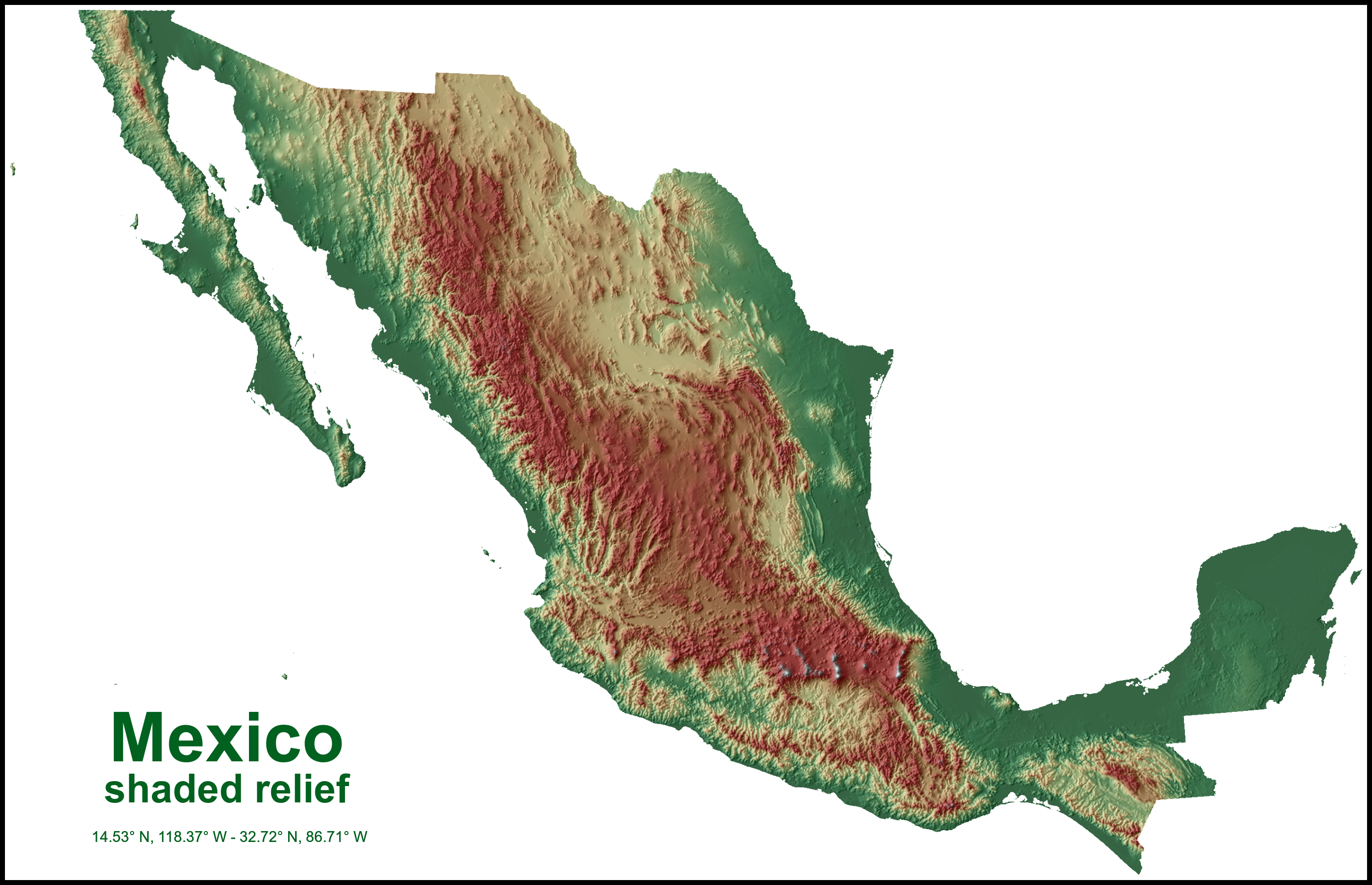 Shaded relief map of Mexico.
In the final map, the tallest peaks can be appreciated in white, such as the Pico de Orizaba (Citlaltépetl), Iztaccihuátl, Nevado de Toluca, Popocatépetl, Cofre de Perote, among others. As a final annotation I was planning to add the altitude range of the map, but the resulting range from the DEM is not very precise, so I decided not to include it (DEM highest point was 5139 m, while highest point should be around 5600 m).