Species occurrence data

The purpose of this post is to download data from GBIF to obtain occurrences registries of a particular species and then to transform that data into a geospatial object and obtain a map.

The first step is to load the required packages. Rgbif is the package that will connect R with the GBIF API, skimr is going to be useful to get a quick view of the data we just downloaded, dply and tidyr will help wrangle and clean the data, rnaturalearth will be used to download a polygon of Mexico’s extent, while sf is going to be used to transform the data into a spatial object (sf) and finally, tmap will be used to make a map.

library(rgbif)
library(skimr)
library(dplyr)
library(tidyr)
library(rnaturalearth)
library(sf)
library(tmap)

The first step will be to set your credentials to be able to acess GBIF. If you do not have these credentials, you can register in their website and obtain them (https://www.gbif.org/user/profile). Then rewrite that information into the R environment

# ---------------1. Set credentials----------------------
# Set credentials
# usethis::edit_r_environ()

# Edit .Renviron
# GBIF_USER="myname"
# GBIF_PWD="mypass"
# GBIF_EMAIL="yeahyeahyeah@myorg.org"

The next step is downloading the data of interest. In this example, I am going to download the data for Rhizhophora mangle in Mexico. You will have to wait for the download to complete. Meanwhile, you can check the status of the download using occ_download_wait and putting in the key of numbers that will appear in the console. Once the download have been finished, you can import the data into R.

# -----------2. Search and download data-----------------
# Now you can use without logging in every session
id <- name_backbone("Rhizophora mangle")$usageKey
# Send download request
occ_download(pred("taxonKey", id),
             pred("country", "MX"),
             format = "SIMPLE_CSV")
# Check status of download
occ_download_wait('key_of_numbers')

# Once finished download to hard drive and save it in df
df <- occ_download_get('key_of_numbers') %>%
  occ_download_import()

Next, you can use skimr to take a look at the general structure of the data and select the columns of interest. Additinoally, you can drop registries without location. (longitude / latitude).

# ---------3. Select vars of interest-------------------
skim(df)

# Select columns of importance
rhizMang <- df |>
  select(scientificName, identifiedBy,
         decimalLatitude, decimalLongitude, coordinateUncertaintyInMeters,
         year, month, day,
         elevation, elevationAccuracy) |>
  # Drop registries without spatial reference
  drop_na(decimalLatitude, decimalLongitude)

Finally, you can transform the data into a spatial object and make a map. Here, I use ne_countries to get the polygon of Mexico and tmap to create the map. Finally, you can export the map.

# ---------4. Geo transformation and map------------------
# Transform into sf object
rhizMang <- st_as_sf(rhizMang, 
                     coords = c("decimalLongitude", "decimalLatitude"),
                     crs = st_crs(4326))

# Get map of Mexico
mx <- ne_countries(scale = 110, 
                   type = "countries", 
                   # continent = NULL,
                   country = "Mexico", 
                   returnclass = c("sf"))

# Do a quick map to see the location of the registries
map1 <- tm_shape(mx) +
  tm_borders() +
  tm_shape(rhizMang) +
  tm_dots(col = "firebrick2", size = 0.05) +
  tm_graticules(lines = F) +
  tm_scale_bar(position = c(0.01,0)) +
  tm_compass(type = "arrow",
             position = c(0.90,0.85))

tmap_save(tm = map1,
          filename = "Plots/Map1.png",
          width = 15,
          height = 10,
          units = "cm",
          dpi = 300)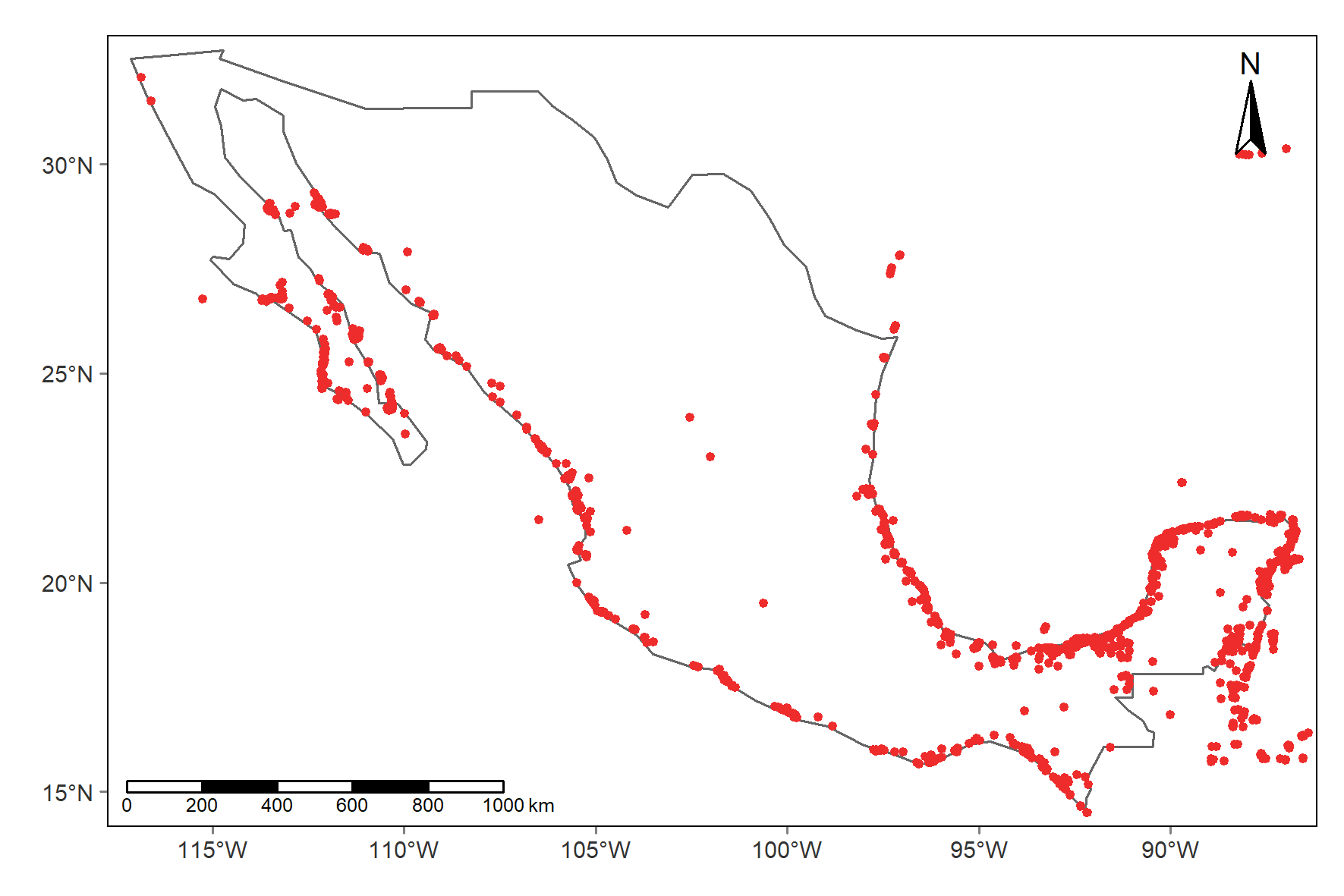

Map with Rhizophora mangle registries in Mexico.