This blog entry will show how to use STAC using R. This example was based on the original STAC tutorial.
First check data providers in the following link Datasets.
Then load necessary packages.
library(sf)
library(rstac)
library(stars)
library(purrr)
In this example we will use Sentinel-2 Collection 1 Level 2A from AWS. Other popular providers are the Microsoft Planetary Computer on https://planetarycomputer.microsoft.com/api/stac/v1. Remember to set the url up to “v1”, i.e., not including the collectino per se.
Define data provider.
stac_source <- rstac::stac(
  "https://earth-search.aws.element84.com/v1"
)
Then, let’s see which collections are available in the endpoint.
col_quer <- stac_source |>
  rstac::collections()
Before running get_request the request is only represented as a future query. Let’s do the request.
available_collections <- rstac::get_request(col_quer)
available_collections
Create a roi or read it from a gpkg file. Need to run at the en st_bbox to be used in the query. Here I created an example roi.
roi <- st_as_sf(tibble::tibble(lat = c(-101.33706520389003,-101.33706520389003,-100.79873512576503, -100.79873512576503, -101.33706520389003),
                        lon = c(19.589466998816956, 20.0674578405529, 20.0674578405529,19.589466998816956, 19.589466998816956)),
         coords = c("lat", "lon"),
         crs = 4326) |>
  st_cast("MULTIPOINT", group_or_split = TRUE) |>
  st_union() |>
  st_cast("POLYGON")

roibbox <- roi |>
  st_bbox()
From the available collections copy and paste the one you are interested in, set the datetime, roi and limit of images.
executed_stac_query <- rstac::stac_search(
  q = stac_source,
  collections = "sentinel-2-c1-l2a",
  bbox = roi,
  datetime = "2021-01-01T00:00:00Z/2021-07-31T23:59:59Z"
) |>
rstac::get_request()
See objects included in query. Check names of bands of interest so they can be used in the download step.
signed_stac_query <- rstac::items_sign(
  executed_stac_query,
  rstac::sign_planetary_computer()
)
signed_stac_query
Download images
folder <- "myfolder"

rstac::assets_download(signed_stac_query,
                       c("nir", "red"),
                       output_dir = folder)
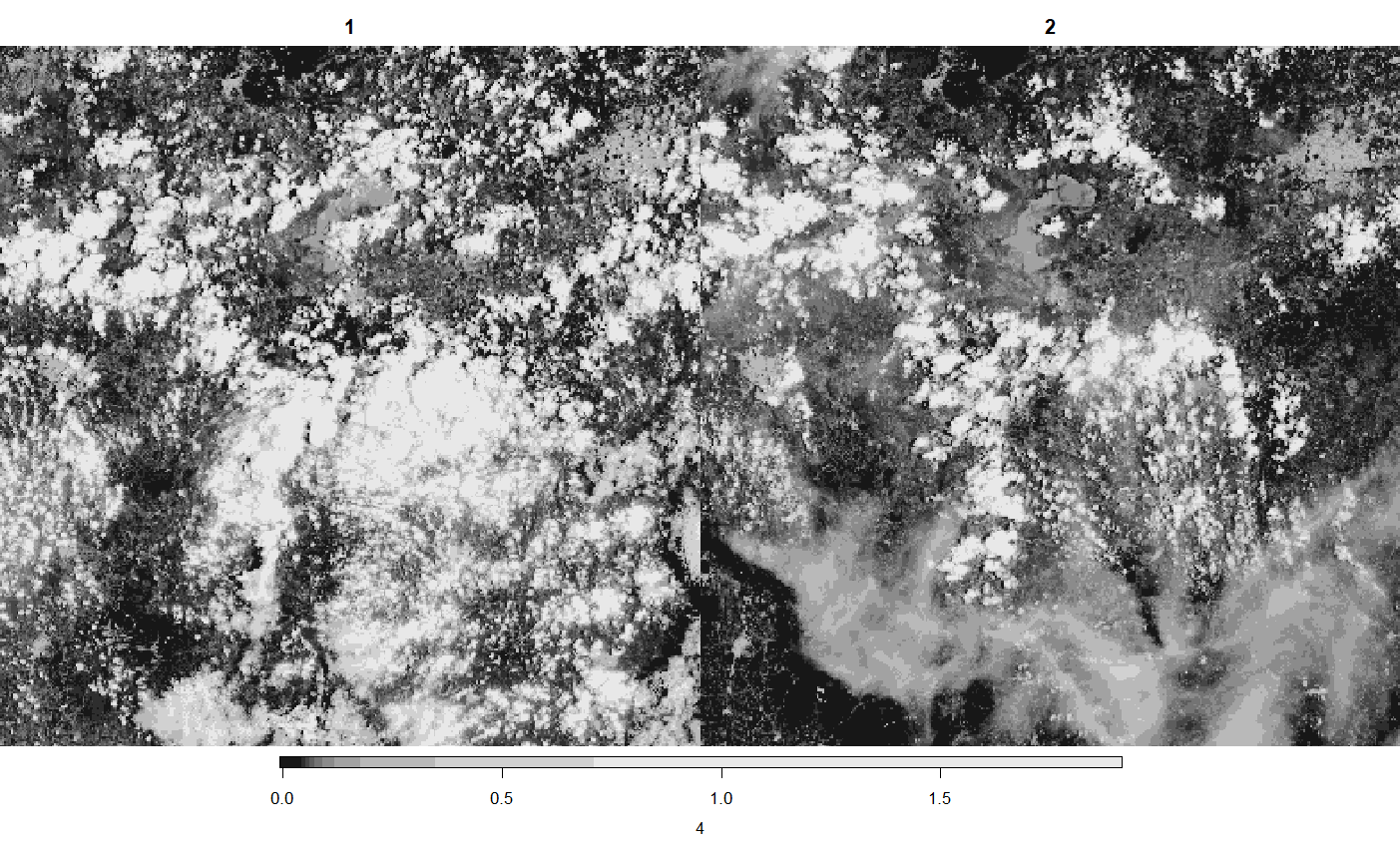
Let’s check the files. We’ll need a loop to stack the two bands for a single date and then create a spatiotemporal object, setting the date as the time dimension. This checking can be done using terra or stars packages. Here we used stars.
Finally, let’s plot the first band in the two available dates.
files <- list.files(folder, "B08|B04", recursive = TRUE, full.names = TRUE)

# Read only first two images (two dates)
imgs <- map(c(1,3), function(i){
  read_stars(files[c(i, (i+1))], proxy = TRUE)
})

# Stack along the time dimension
imgs2 <- do.call(c, c(imgs, along = "time"))

# See result
plot(imgs2[1,,,1:2])