Wordclouds in R

Wordclouds are a great way of visualizing the most frequent terms in texts. Additionally, R provides some great tools to convert pdfs into text files and clean the texts, so non-informative terms are ignored (e.g., articles, prepositions, etc.).

Converting data from pdf to text

library(pdftools)
library(wordcloud)
library(tm)
library(tidyverse)


# Convert pdf 2 text function
files <- list.files("pdf/",
                    "*.pdf",
                    full.names = T)
pdfs <- sapply(files, function(x){
  pdftools::pdf_text(x) %>%
    paste(sep = " ") %>%
    # Remove special characters
    stringr::str_replace_all(fixed("\n"), " ") %>%
    stringr::str_replace_all(fixed("\r"), " ") %>%
    stringr::str_replace_all(fixed("\t"), " ") %>%
    stringr::str_replace_all(fixed("\""), " ") %>%
    paste(sep = " ", collapse = " ") %>%
    stringr::str_squish() %>%
    stringr::str_replace_all("- ", "") 
})

# Clean text by removing numbers, spaces, punctuation, etc.
arts_text_clean <- Corpus(VectorSource(pdfs))

# Remove punctutation
arts_text_clean <- tm_map(arts_text_clean, removePunctuation)
# Pass all word to lowercase
arts_text_clean <- tm_map(arts_text_clean, content_transformer(tolower))
# Remove numbers
arts_text_clean <- tm_map(arts_text_clean, removeNumbers)
# Remove spaces
arts_text_clean <- tm_map(arts_text_clean, stripWhitespace)
# Remove stopwords
arts_text_clean <- tm_map(arts_text_clean, removeWords, stopwords('english'))
arts_text_clean <- tm_map(arts_text_clean, removeWords, stopwords('spanish'))
arts_text_clean <- tm_map(arts_text_clean, removeWords, stopwords('portuguese'))

# Create matrix
arts_text_clean <- TermDocumentMatrix(arts_text_clean) 
arts_text_clean <- as.matrix(arts_text_clean) 
arts_text_clean <- sort(rowSums(arts_text_clean),decreasing=TRUE) 
df <- data.frame(word = names(arts_text_clean),freq=arts_text_clean)

# Remove leftover punctuations and words that wish to be omitted
df <- df |>
  # Need to add the freq as I can't remove the hyphen
  filter(word != "–" & word != "−" & word != "•" & freq != 466 &
           word != "crossref" & word != "doi" & word != "thus" & word != "two" &
           word != "one" & word != "fig" & word != "three" & word != "can" & 
           word != "may" & word != "therefore" & word != "first" & word != "also" &
           word != "author" & word != "journal" & word != "among" & word != "figure" &
           word != "solórzano" & word != "gallardocruz" & word != "jiménezlópez" &
           word != "springer" & word != "although" & word != "however" & word != "authors") |>
  mutate_at(vars(word), function(x) ifelse(x == "ecol", "ecology", x)) |>
  mutate_at(vars(word), function(x) ifelse(x == "sens", "sensing", x)) |>
  mutate_at(vars(word), function(x) ifelse(x == "environ", "environment", x)) |>
  group_by(word) |>
  summarise(freq2 = sum(freq))

Wordcloud

To do the wordcloud you will need a dataframe containing the words and its corresponding frequency of appearance. In this case that object is saved as df and contains two columns word and freq2. The rest of the arguments let you choose the minimum frequency shown in the wordplot, the maximum number of words shown in the plot, if a random order should be used, rotation percentage and the colors of the words.

set.seed(1234) # for reproducibility 

png("wordcloud.png",
    width = 10,
    height = 10,
    units = "cm",
    res = 300)
wordcloud(words = df$word, 
          freq = df$freq2, 
          scale=c(3.5,0.25),
          min.freq = 20,
          max.words=200, 
          random.order=FALSE, 
          rot.per=0.35,
          colors=rev(brewer.pal(6, "Dark2")))
dev.off()

An example of a wordplot.

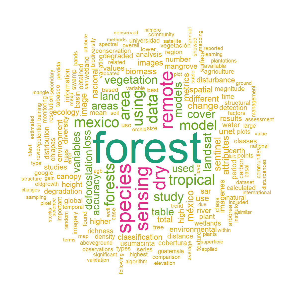Wordcloud of my publications.