DEM as ridgelines in R

DEM as ridgelines in R

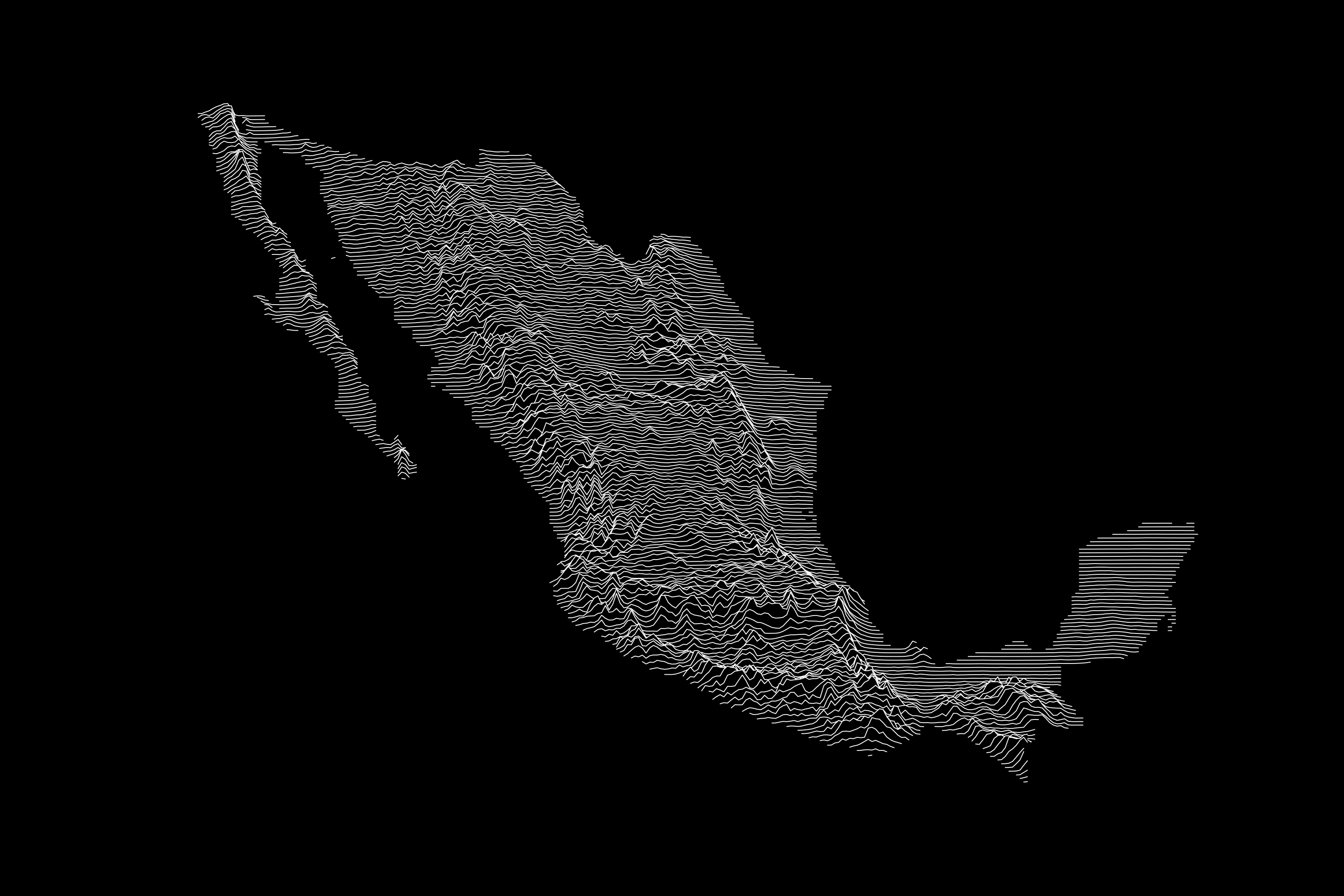
This post will show you how to visualize a DEM as a ridgeline plot, similar to the famous Joy Division - Unkown Pleasures album cover. This post was based on the original post of DiegHernan at: https://dieghernan.github.io/202205_Unknown-pleasures-R/ with only minor modifications

First, install and load packages

library(sf)
library(terra)
library(elevatr)
# Need to install from remotes to work
# remotes::install_github("ropensci/rnaturalearthdata")
library(rnaturalearth)
library(tidyverse)
library(ggridges)

Area of interest

In this exmample, we are going to use rnaturalearth to download the polygon of a country of interest, so this can be used to afterwards obtain the DEM for this polygon.

region <- ne_countries(country = "Mexico", 
                       scale = "medium", 
                       returnclass = "sf") |>
  st_transform(6372)

Get elevation data

Get DEM data using z values depending on the desired zoom (higerh value: more zoom) and extent of the area of interest. Convert to rast and mask using the polygon.

dem <- get_elev_raster(location = region, 
                       z = 6, 
                       prj = st_crs(region),
                       src = "aws",
                       clip = "bbox", 
                       expand = 2000) 
dem <- rast(dem) |>
  mask(vect(region)) 

dim(dem)
plot(dem)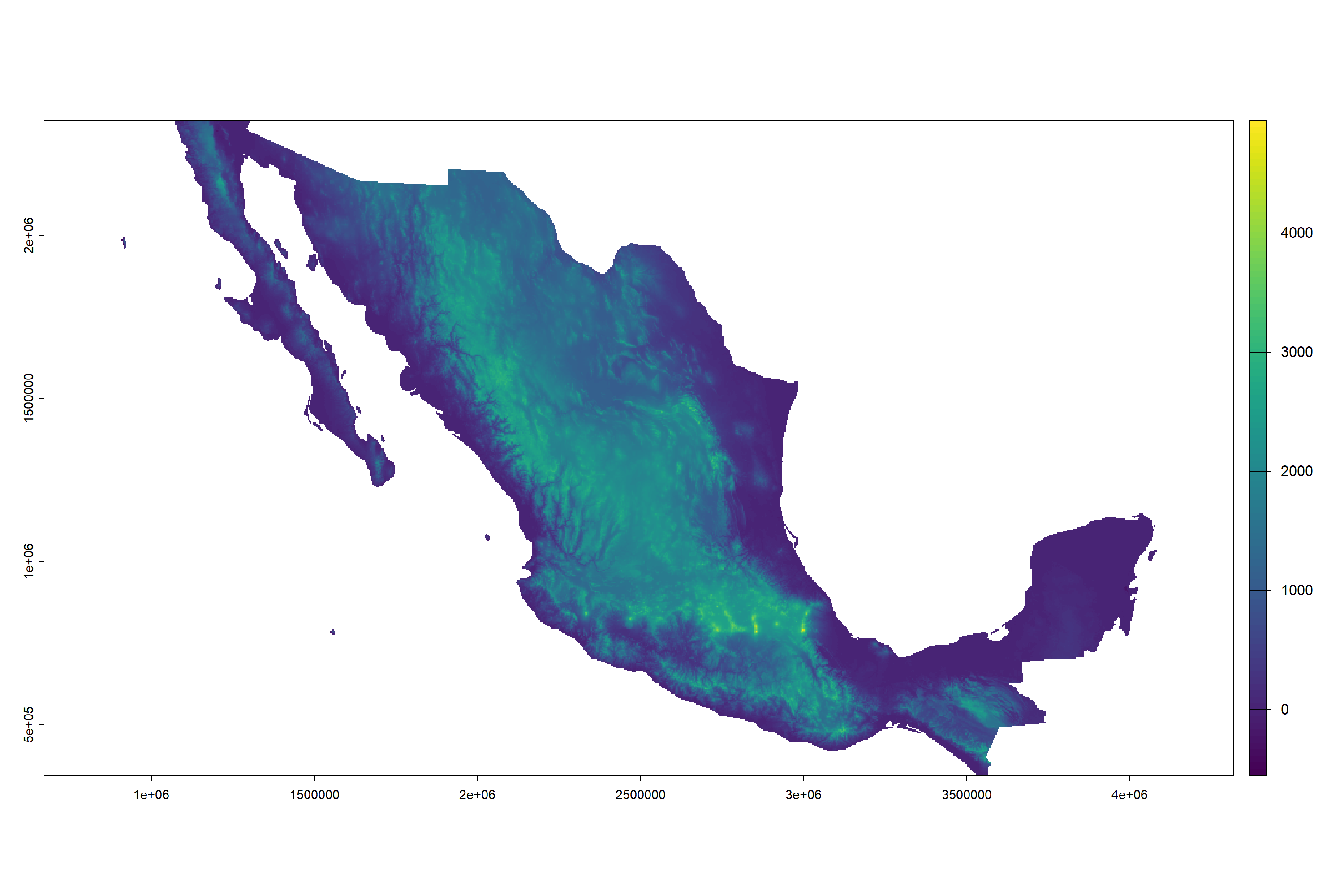

Mexico DEM

If image has very high resolution, aggregate by a selected factor. In this case, reduce the pixel resolution by a factor of 10.

dem_lowres <- aggregate(dem, 10)
names(dem_lowres) <- "elevation"

dim(dem_lowres)
plot(dem_lowres)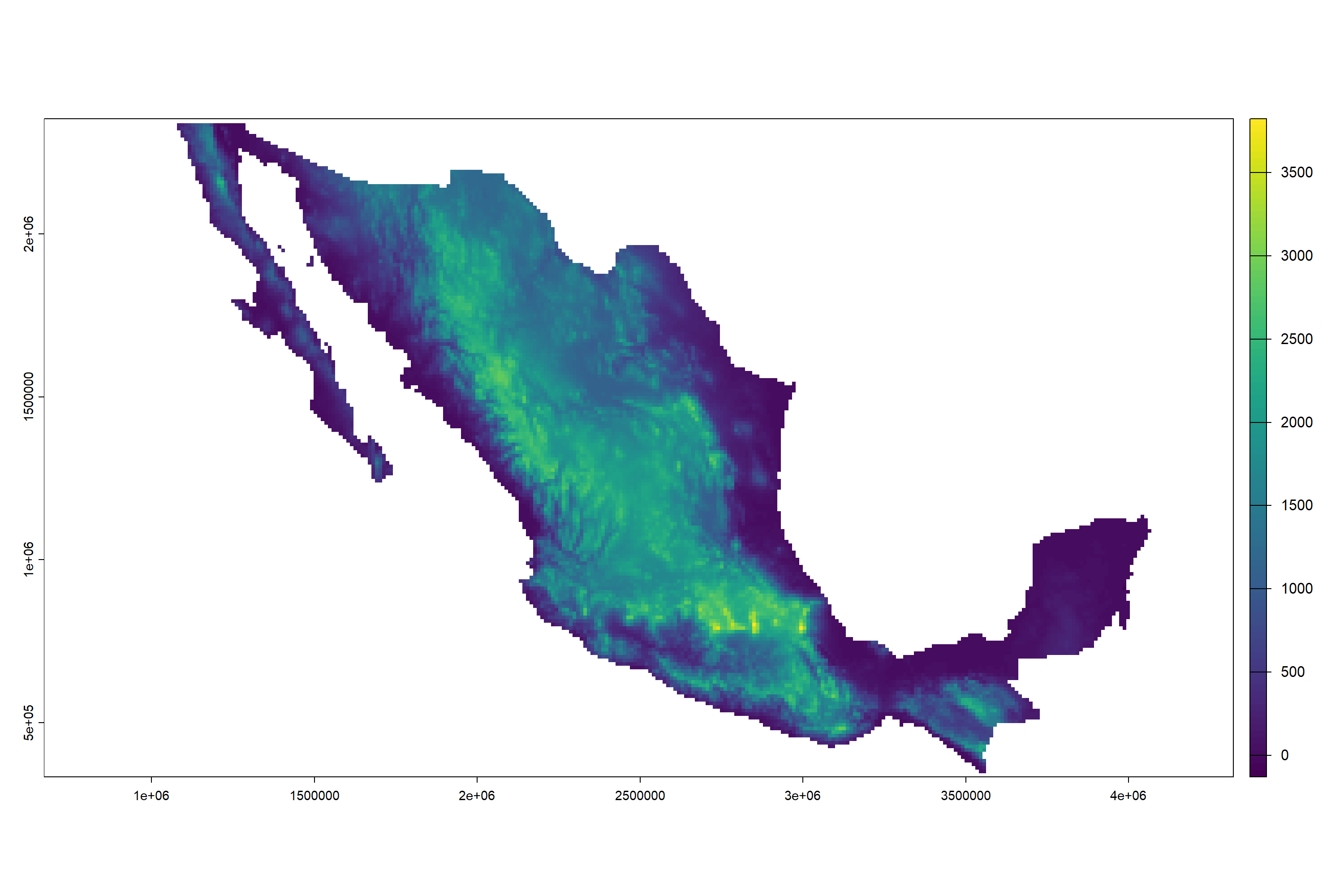

Mexico DEM low resolution

Then transform the DEM into a table format so it can be ingested into ggplot.

dem_df <- as.data.frame(dem_lowres, xy = TRUE, na.rm = FALSE)

Create the ridges plot. Add the sf object as the base layer, then add on top, the ridgeline plot. You can change the colors (color: color of the line, fill: color of the space between lines), lwd (width of lines) and scale (factor by which to scale z values) to get the best visual result.

ggplot() +
  geom_sf(data = region, 
    color = NA, 
    fill = "black", 
    alpha = 0.95) +
  geom_ridgeline(
    data = dem_df, aes(
      x = x, 
      y = y,
      group = y,
      height = elevation
    ),
    scale = 25,
    fill = "black",
    color = "white",
    lwd = 0.25,
    min_height = 0.1
  ) +
  theme_void() +
  theme(plot.background = element_rect(fill = "black"))

Mexico DEM low resolution